Wrangling Census data 🇨🇦
Last updated on
Welcome to this new exciting project! We will tap into the vast trove of information from the Canadian Census provided by Statistics Canada! To crunch the data, we will use the Simple Data Analysis library (SDA), which I created (give it a ⭐ ).
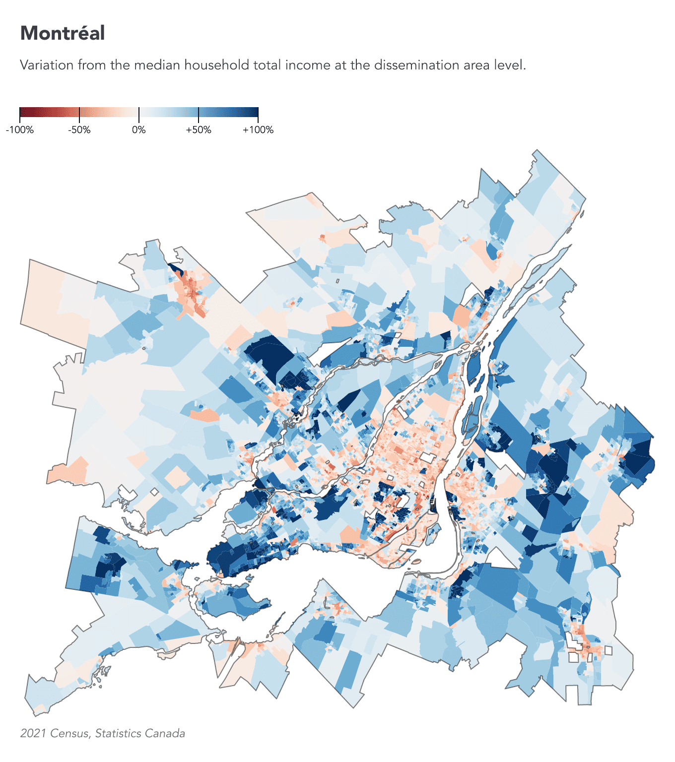
For each metropolitan area, we will create a map showing areas with lower or higher income levels. The Montréal map below is an example of the final output we’ll achieve together.
In this real-world project, I will show you advanced techniques for crunching large datasets with TypeScript. The 2021 Census data is approximately 30 GB, but you will actually need about 70 GB of free space on your hard drive for this project. Time to do some cleaning! 🧹
If you are stuck at any point in this project, it may be beneficial to review the previous lessons explaining the basics of SDA:
We will use Node.js and VS Code. Make sure you’ve gone through the Setup lesson as well.
Let’s get started!
What’s the question?
To avoid getting lost, let’s define the question we’re trying to answer:
- For each Canadian metropolitan area, which dissemination areas have household incomes above or below the median?
The metropolitan areas are defined as follows in the Census:
A census metropolitan area (CMA) is formed by one or more adjacent municipalities centred on a population centre (known as the core). A CMA must have a total population of at least 100,000, of which 50,000 or more must live in the core.
And here’s the definition of dissemination areas:
A dissemination area (DA) is a small, relatively stable geographic unit with an average population of 400 to 700 persons. It is the smallest standard geographic area for which all census data are disseminated. DAs cover all the territory of Canada.
Let’s code!
Setup
Create a new empty folder somewhere handy on your computer and open it in VS Code. Then open the terminal in VS Code.
We’ll use @nshiab/setup-data-project, a library I created to install the libraries and set up all the files and configuration we need for a project. Run this command in the terminal:
npx @nshiab/setup-data-project --sdaIf prompted to install the library, type y and press Enter.
The --sda option automatically selects the simple-data-analysis library for installation.
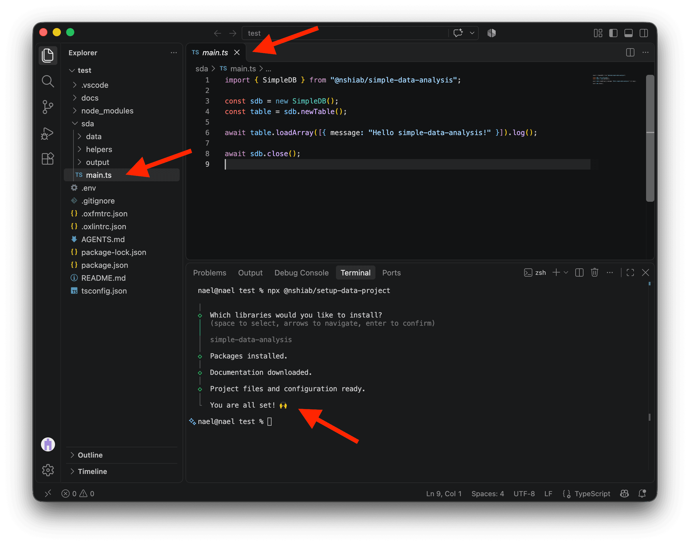
Once the terminal says You are all set!, open sda/main.ts. You’ll see some starter code in it.
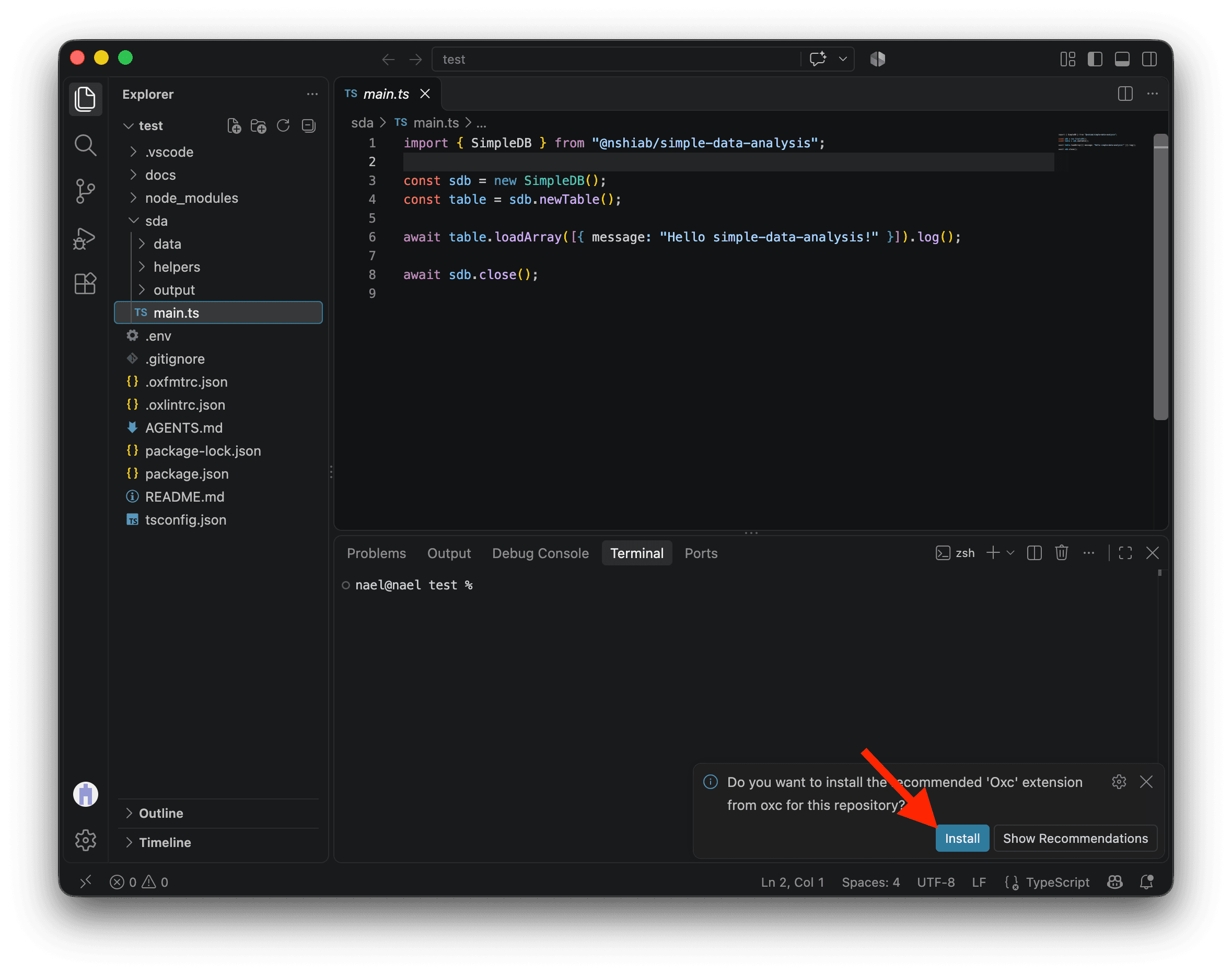
If VS Code asks you to install the recommended Oxc extension, click Install. It helps format your code and find potential problems as you work.
We’re now ready to watch sda/main.ts. Run the command below. Every time you save the file, it will automatically format, check, and run your code:
npm run sda:watchIf you ever need to stop watching, click the terminal and press Ctrl+C on Mac or Windows.
Keep the watcher running while you work through this lesson.
Downloading the data
To download the Census data with the most granularity, click on this Statistics Canada page .
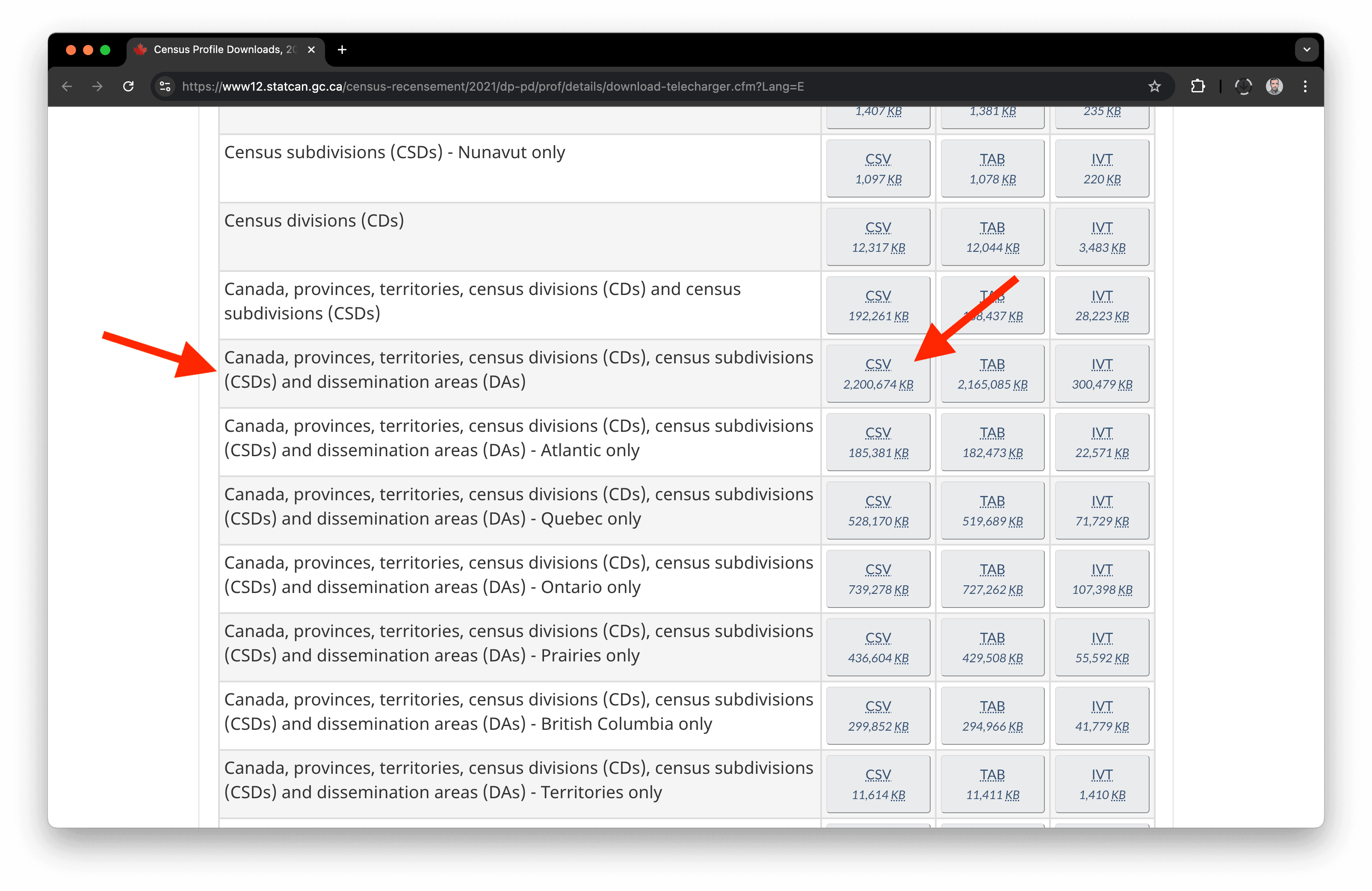
Click on the first drawer Comprehensive download file and then on the CSV button for Canada, provinces, territories, census divisions (CDs), census subdivisions (CSDs), and dissemination areas (DAs).
In case you can’t find it, here’s the direct link . This will download a 2.25 GB zip file.
Because we want to work on the metropolitan areas, it would be great to have the metropolitan area names for each dissemination area.
Statistics Canada provides this information in the 2021 Geographic Attribute File . Download it from this direct Statistics Canada link . It is a 9.8 MB zip file named 2021_92-151_X.zip.
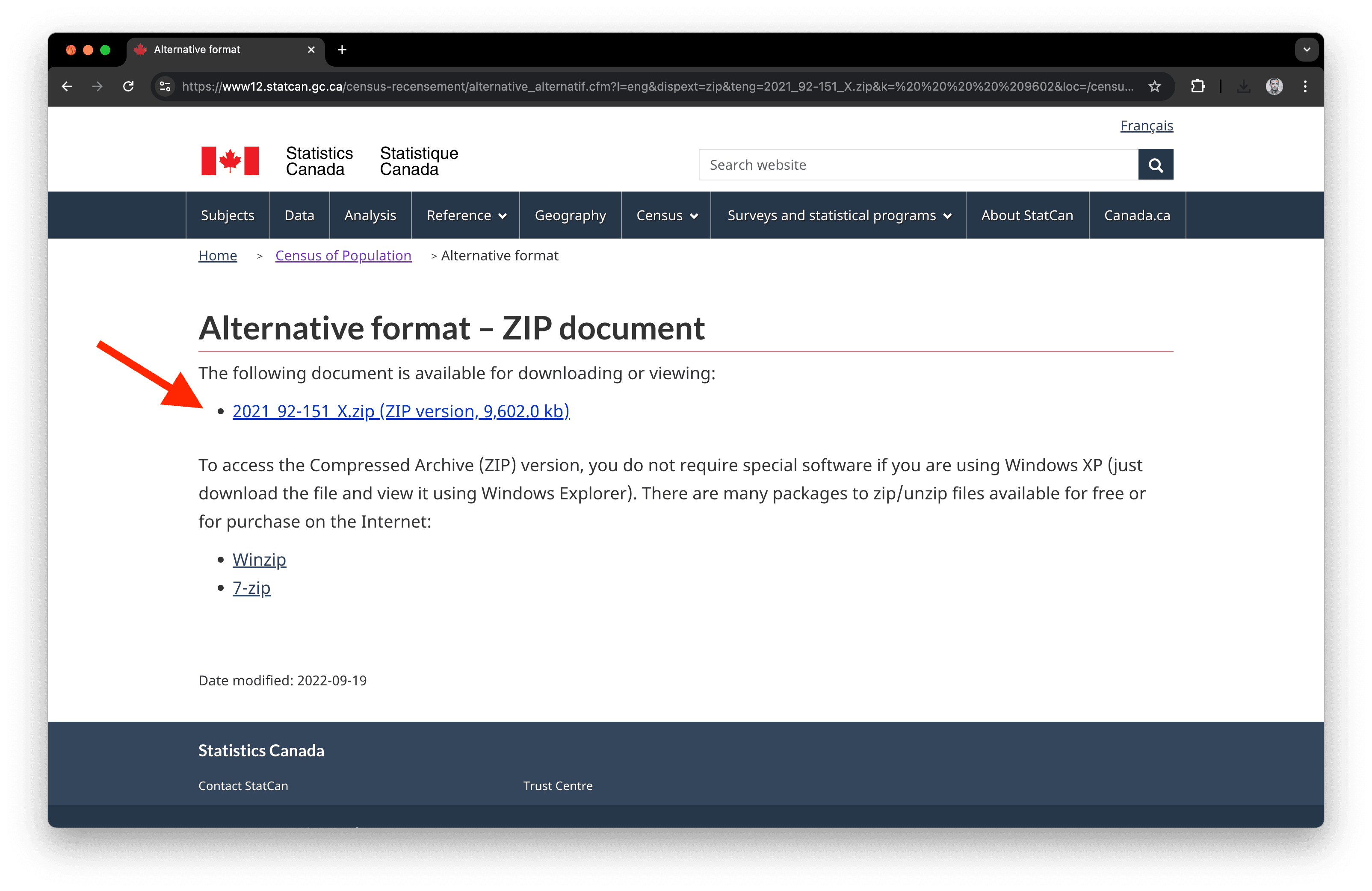
And finally, since we want to create a map, we need the geospatial boundaries of the dissemination areas. You’ll find them here .
Click on the drawer Statistical boundaries and select Dissemination areas. In the Format section, select Shapefile, then hit Continue at the bottom of the page.
In case you can’t find it, here’s the direct link to download the file. It’s around 197 MB.
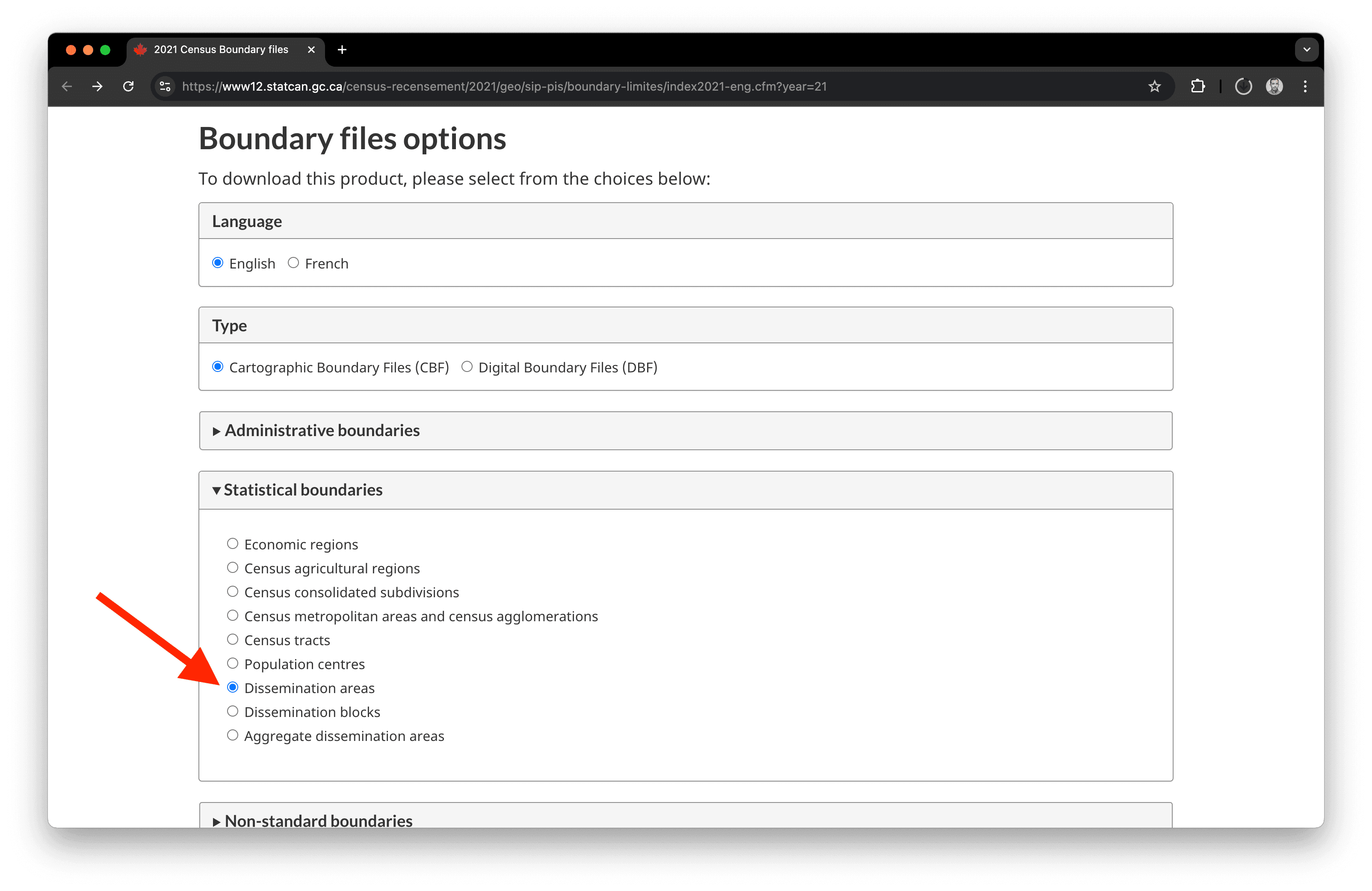
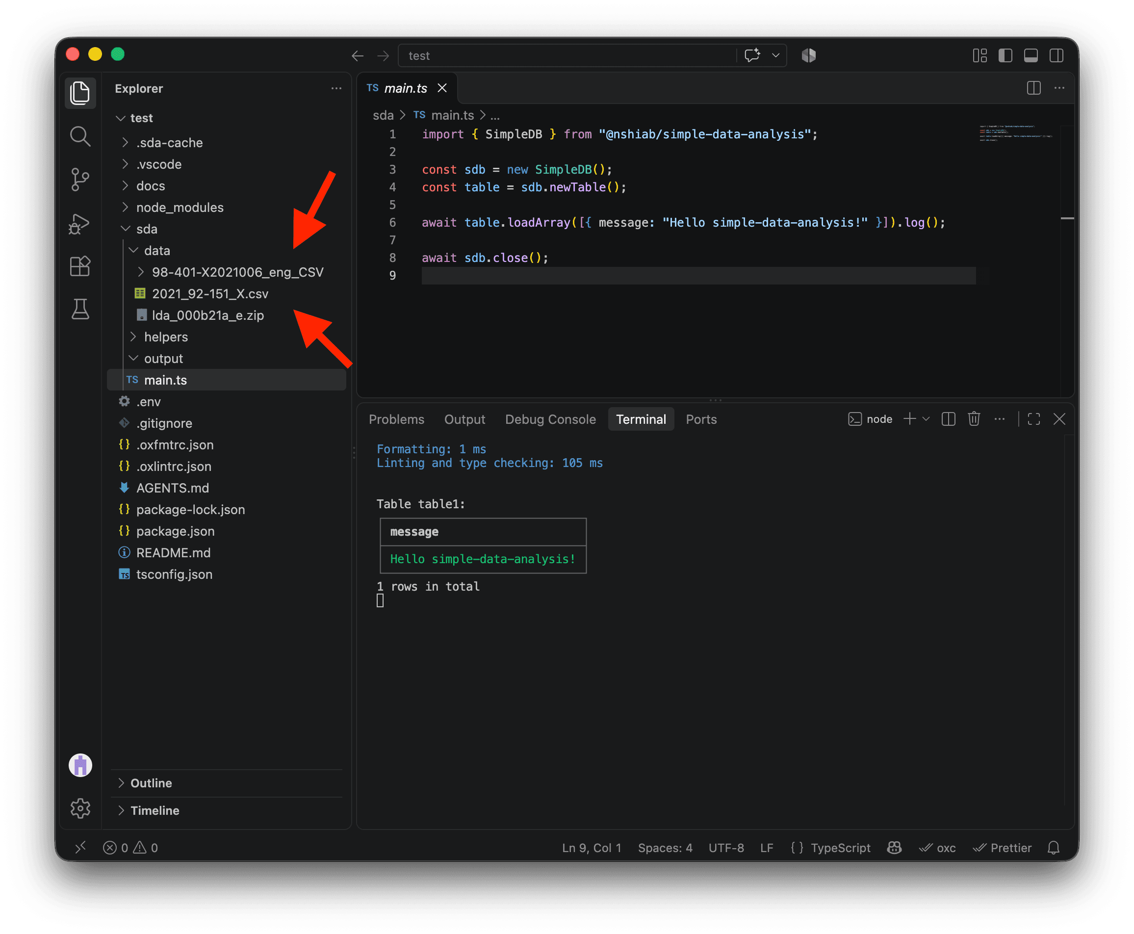
Now, move all of this inside the data folder in your project and unzip everything except the geospatial boundaries in the file lda_000b21a_e.zip!
To unzip, check your folder outside of VS Code, like in Finder or File Explorer. You might need software like Winzip or 7-zip. Once unzipped, remove the two original .zip files from your project and download folder, and don’t forget to empty your trash! 🗑️ Disk storage is precious when you work with big datasets.
Surprise! You now have over 27 GB of data waiting to be processed. 😅
The Census data
Loading what we need
When we unzipped the census data, we got a folder with multiple files in it. The data is in the files with the _data_ substring.
Let’s try to load the first 1,000 rows of the first file, for the Atlantic provinces. These files are very large, so we’ll use the limit option to load just a sample while exploring them.
import { SimpleDB } from "@nshiab/simple-data-analysis";

const sdb = new SimpleDB();

await sdb
  .newTable("census")
  .loadData(
    "sda/data/98-401-X2021006_eng_CSV/98-401-X2021006_English_CSV_data_Atlantic.csv",
    { limit: 1000 },
  ).log();

await sdb.close();
Hmmm… We have a problem. This error means that the data is not using the UTF-8 encoding, which is the standard nowadays.
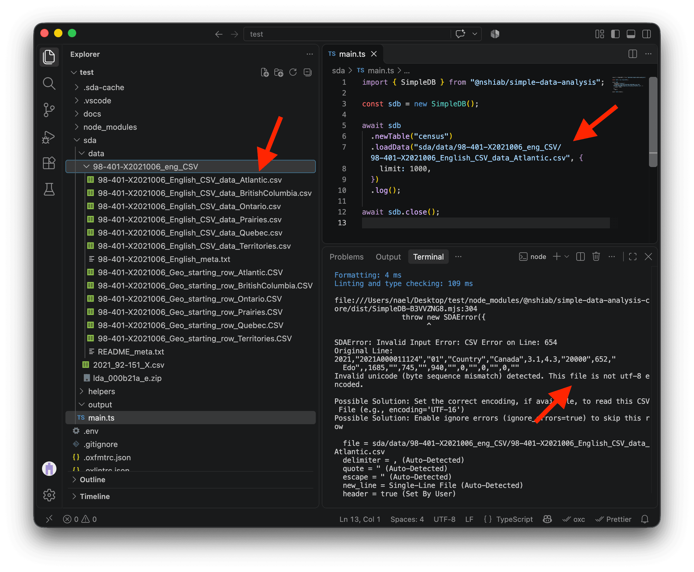
The Atlantic CSV has a long path. To copy it without typing it out, right-click the file in VS Code’s Explorer and select Copy Relative Path.
I asked Statistics Canada about this, and they told me they use the Windows-1252 encoding. Luckily, SDA has an encoding option. We can use cp1252 to refer to this encoding, and SDA will automatically convert the data to UTF-8 behind the scenes.
Update your code with the example below and save the file (COMMAND + S on Mac or CTRL + S on Windows). The first 1,000 rows should now appear.
import { SimpleDB } from "@nshiab/simple-data-analysis";

const sdb = new SimpleDB();

await sdb
  .newTable("census")
  .loadData(
    "sda/data/98-401-X2021006_eng_CSV/98-401-X2021006_English_CSV_data_Atlantic.csv",
    { limit: 1000, encoding: "cp1252" },
  ).log();

await sdb.close();
Amazing! It works! 🥳
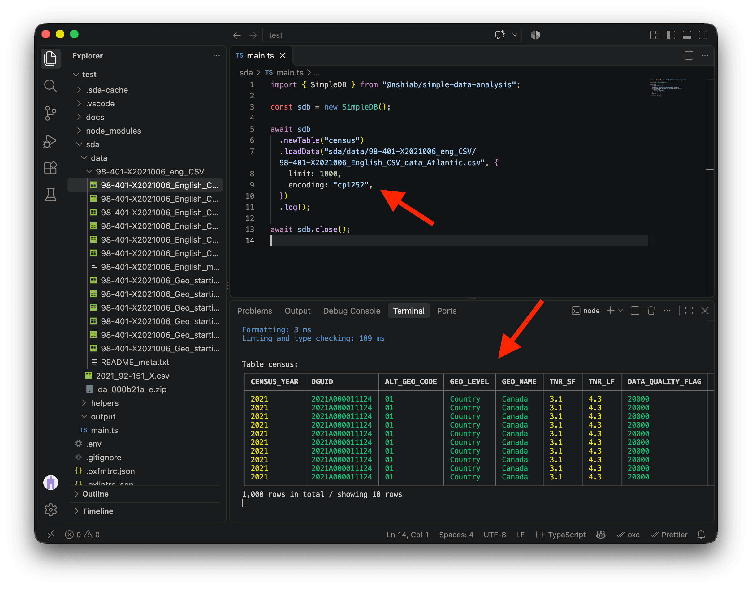
If the table layout is displayed weirdly in your terminal, it’s because the width of the table is bigger than the width of your terminal. Right-click on the terminal and look for Toggle size with content width. There is also a handy shortcut that I use all the time to do that: OPTION + Z on Mac and ALT + Z on PC.
We can see a lot of columns in our data, but we only need four from the CSV file:
GEO_LEVEL: The type of geographic area represented by the row.CHARACTERISTIC_ID: The Census variable represented by the row.DGUID: The unique geographic identifier we will use to join our data.C1_COUNT_TOTAL: The value of the Census variable.
We can use the columns option to load only these four columns.
import { SimpleDB } from "@nshiab/simple-data-analysis";

const sdb = new SimpleDB();

await sdb
  .newTable("census")
  .loadData(
    "sda/data/98-401-X2021006_eng_CSV/98-401-X2021006_English_CSV_data_Atlantic.csv",
    {
      limit: 1000,
      encoding: "cp1252",
      columns: ["GEO_LEVEL", "CHARACTERISTIC_ID", "DGUID", "C1_COUNT_TOTAL"],
    },
  ).log();

await sdb.close();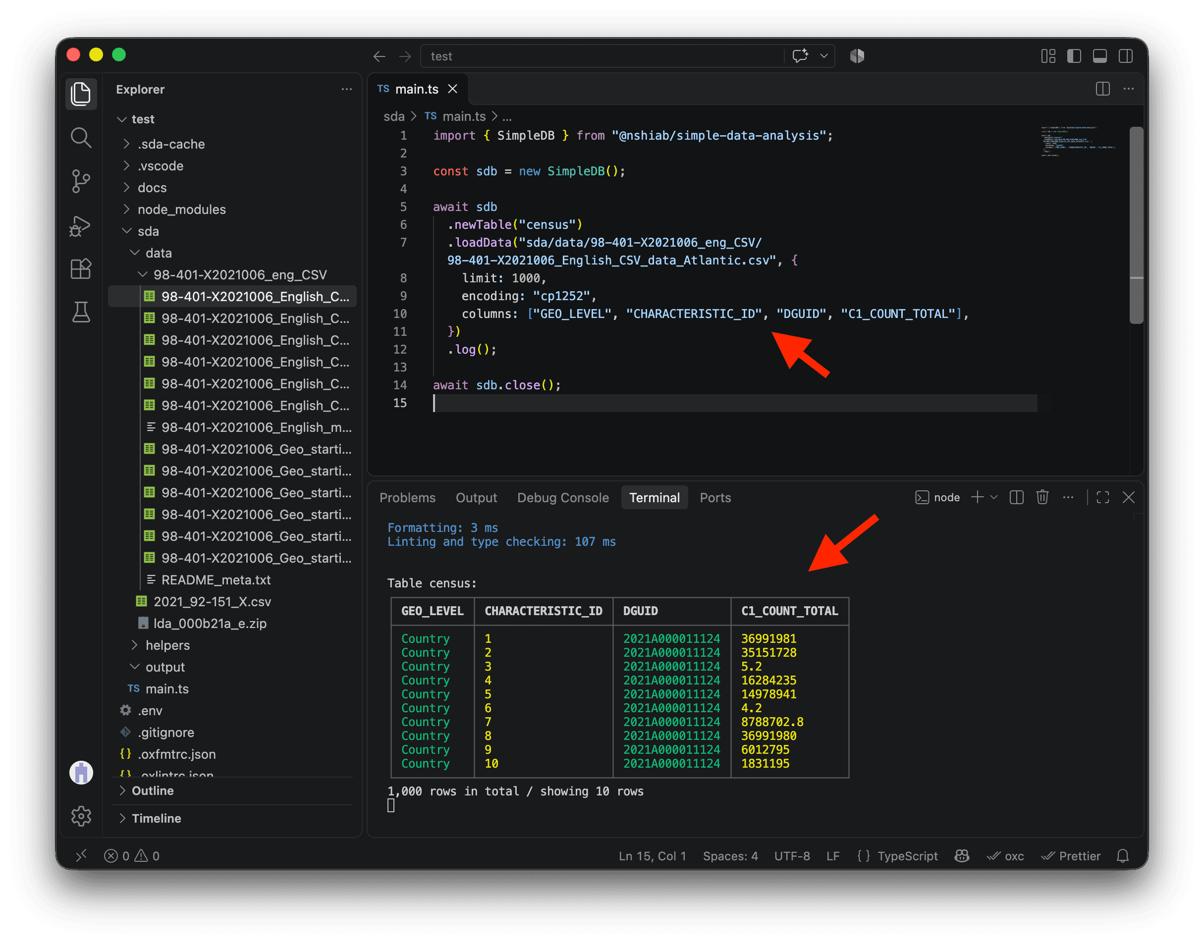
The GEO_LEVEL column currently shows country-level rows. That’s because the file we downloaded contains Canada, provinces, territories, census divisions, census subdivisions, and dissemination areas, while we only need dissemination areas.
We can use the conditions option to keep only dissemination area rows in our table.
import { SimpleDB } from "@nshiab/simple-data-analysis";

const sdb = new SimpleDB();

await sdb
  .newTable("census")
  .loadData(
    "sda/data/98-401-X2021006_eng_CSV/98-401-X2021006_English_CSV_data_Atlantic.csv",
    {
      limit: 1000,
      encoding: "cp1252",
      columns: ["GEO_LEVEL", "CHARACTERISTIC_ID", "DGUID", "C1_COUNT_TOTAL"],
      conditions: `GEO_LEVEL = 'Dissemination area'`,
    },
  ).log();

await sdb.close();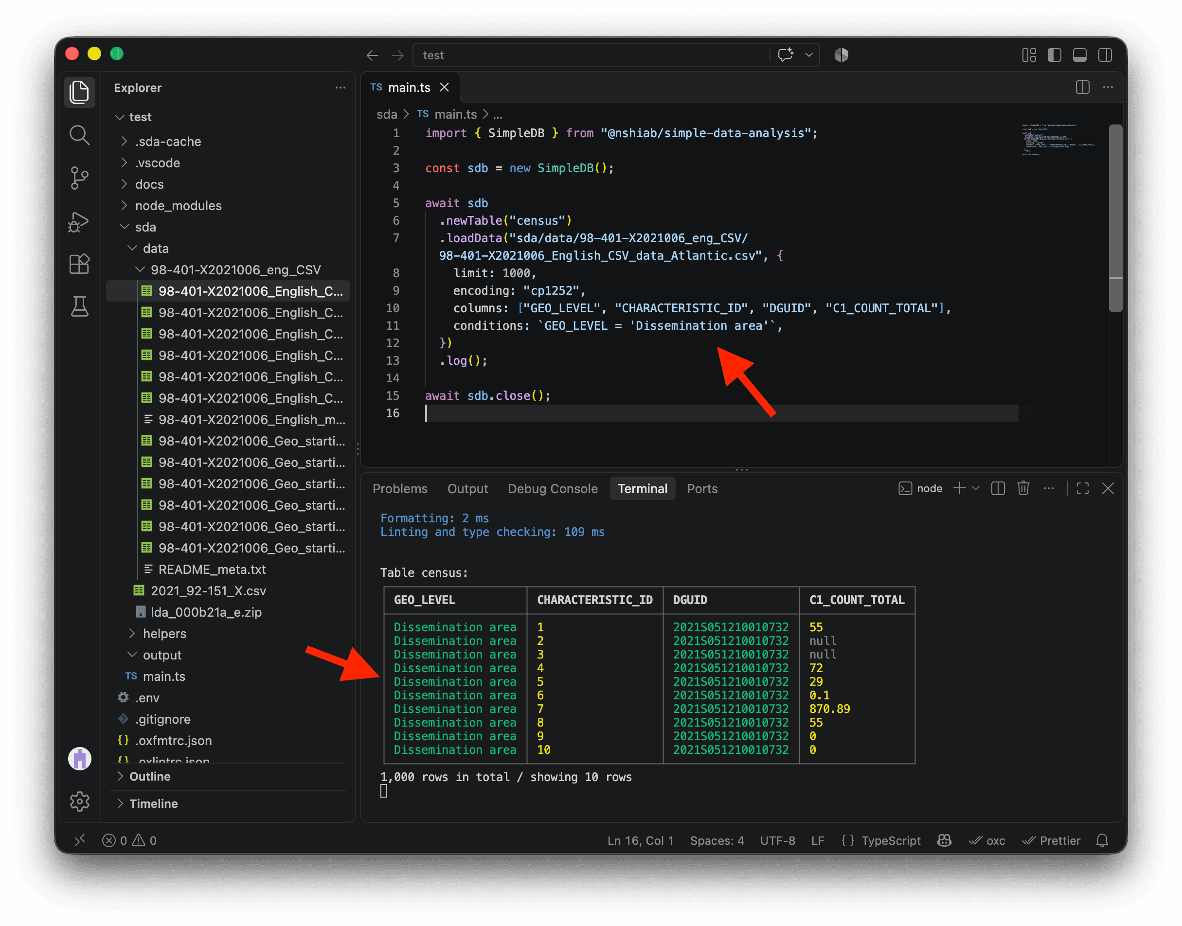
We are now ready to remove the limit option and load all the data from the Atlantic CSV file. Before doing that, let’s use the cache method and enable cacheVerbose to see more details in the terminal about how and what SDA caches.
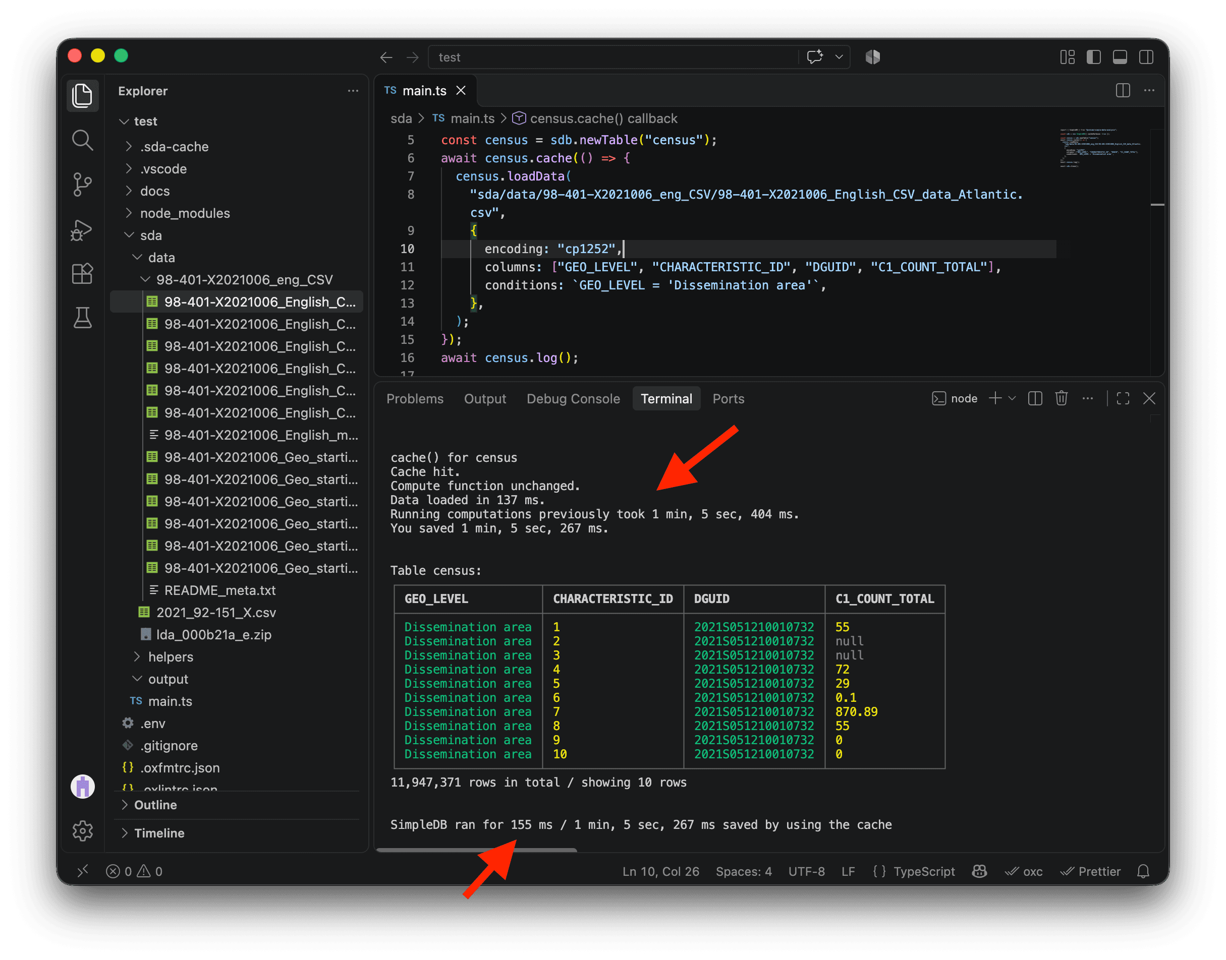
On the first run, cache runs the code we pass it and saves the resulting table in a new .sda-cache folder. On subsequent runs, unchanged code loads the result directly from the cache instead of reading the original file again, converting its encoding, selecting its columns, and filtering its rows. This is much faster.
import { SimpleDB } from "@nshiab/simple-data-analysis";

const sdb = new SimpleDB({ cacheVerbose: true });

const census = sdb.newTable("census");
await census.cache(() => {
  census.loadData(
    "sda/data/98-401-X2021006_eng_CSV/98-401-X2021006_English_CSV_data_Atlantic.csv",
    {
      encoding: "cp1252",
      columns: ["GEO_LEVEL", "CHARACTERISTIC_ID", "DGUID", "C1_COUNT_TOTAL"],
      conditions: `GEO_LEVEL = 'Dissemination area'`,
    },
  );
});
await census.log();

await sdb.close();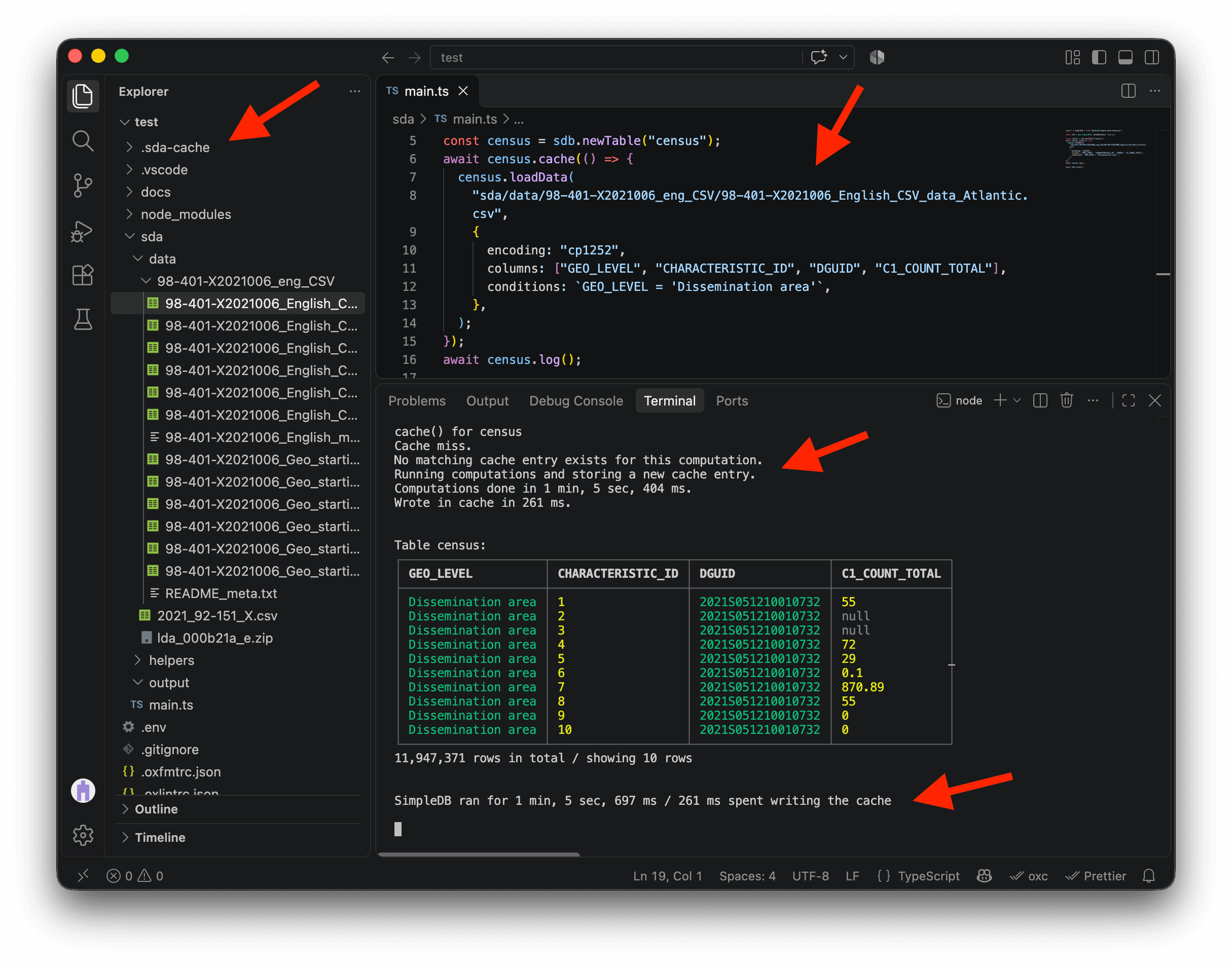
On my machine, loading nearly 12 million rows took about 1 minute and 6 seconds and created a new .sda-cache folder. To be honest, that’s pretty slow for SDA. Most of that time went into converting the CSV from Windows-1252 to UTF-8. Loading can be much faster when the data is already in UTF-8. On the same M4 Max, I loaded a billion rows in about eight seconds for the One Billion Row Challenge 😱. If you haven’t tried it yet, give it a go after this project.
Save main.ts again without changing the code inside cache (COMMAND + S on Mac or CTRL + S on Windows). SDA will load the data directly from .sda-cache. On my machine, the full run took just 155 milliseconds with the cache, about 424 times faster than the first run, which took 1 minute, 5 seconds and 697 milliseconds. That’s the beauty of caching! ⚡
To clear all cached data, run npm run clean. This removes both .sda-cache and .tmp. You can also delete either folder manually.
It is now time to load the Census data for all provinces and territories. If you look at the CSV files, their names all follow the same pattern: 98-401-X2021006_English_CSV_data_[region].csv.
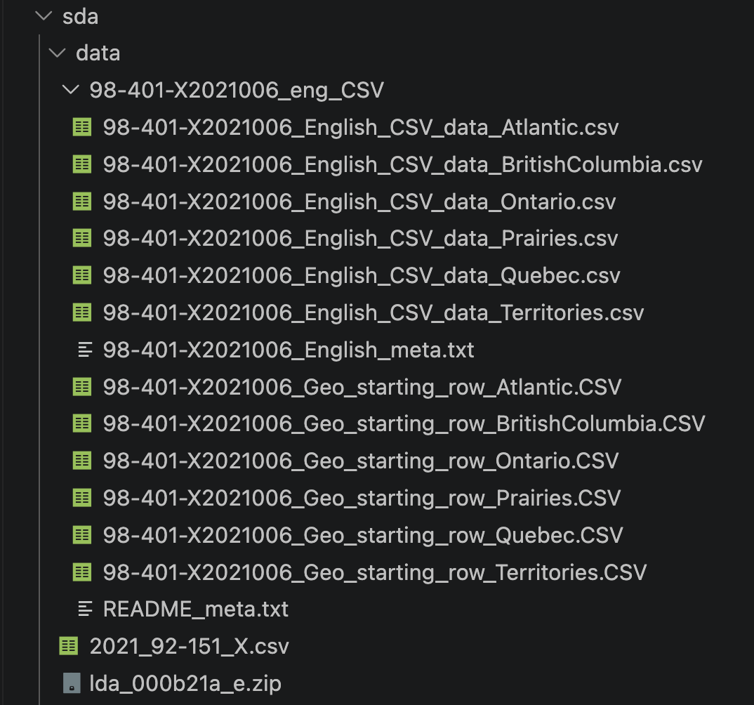
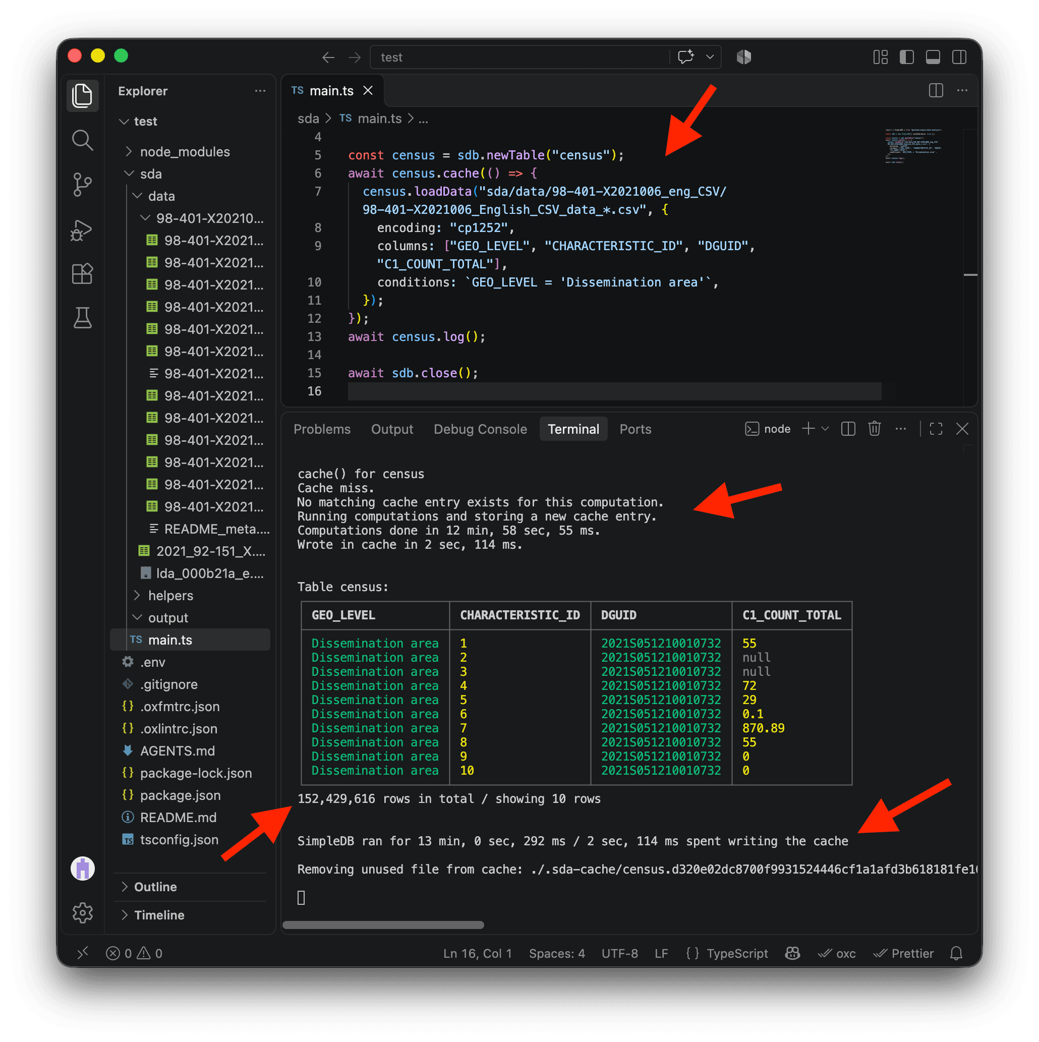
We can replace Atlantic in the path with the wildcard *. SDA will load 98-401-X2021006_English_CSV_data_Atlantic.csv, 98-401-X2021006_English_CSV_data_BritishColumbia.csv, and all the other CSV files whose paths follow the same pattern. They will all be loaded directly into the census table. Very handy! 🎉
⚠️ The code below will load millions and millions of rows. Depending on how powerful your machine is, it might take a long time. Update the code, save main.ts, and be patient while it runs.
import { SimpleDB } from "@nshiab/simple-data-analysis";

const sdb = new SimpleDB({ cacheVerbose: true });

const census = sdb.newTable("census");
await census.cache(() => {
  census.loadData(
    "sda/data/98-401-X2021006_eng_CSV/98-401-X2021006_English_CSV_data_*.csv",
    {
      encoding: "cp1252",
      columns: ["GEO_LEVEL", "CHARACTERISTIC_ID", "DGUID", "C1_COUNT_TOTAL"],
      conditions: `GEO_LEVEL = 'Dissemination area'`,
    },
  );
});
await census.log();

await sdb.close();
On my machine, this first run took roughly 13 minutes. Most of that time was spent converting the data from Windows-1252 to UTF-8, rather than reading the CSV files. The result is now cached, so I will not have to wait that long when I run the same code again. We now have more than 152 million rows of data in our table! 🤭
Depending on the RAM available on your computer, you might see a .tmp folder appear in your project. If the data is bigger than your RAM, SDA uses this folder to store processed chunks while it works. The folder can become quite big. You can remove .tmp manually, although I usually don’t bother. Running npm run clean will remove it too, but be careful: it will also delete all cached data in .sda-cache.
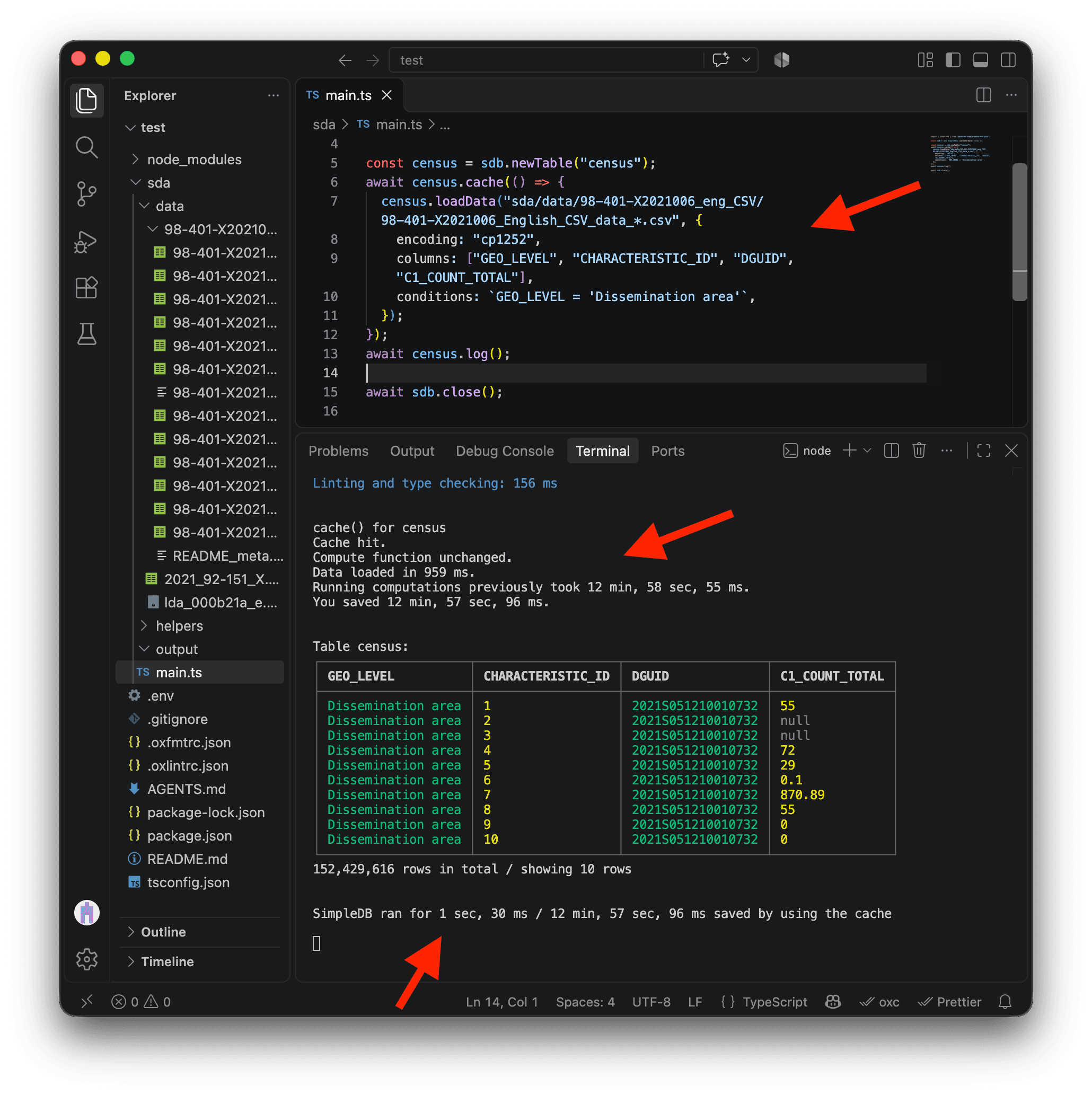
Save main.ts again or rerun the script without changing the code inside cache. On my machine, the full run with the cache took just 1 second and 30 milliseconds, about 758 times faster than the first run. Absolutely stunning speed! 😎
Filtering the Census variables
Let’s refresh our memory. Our question is:
- For each Canadian metropolitan area, which dissemination areas have household incomes above or below the median?
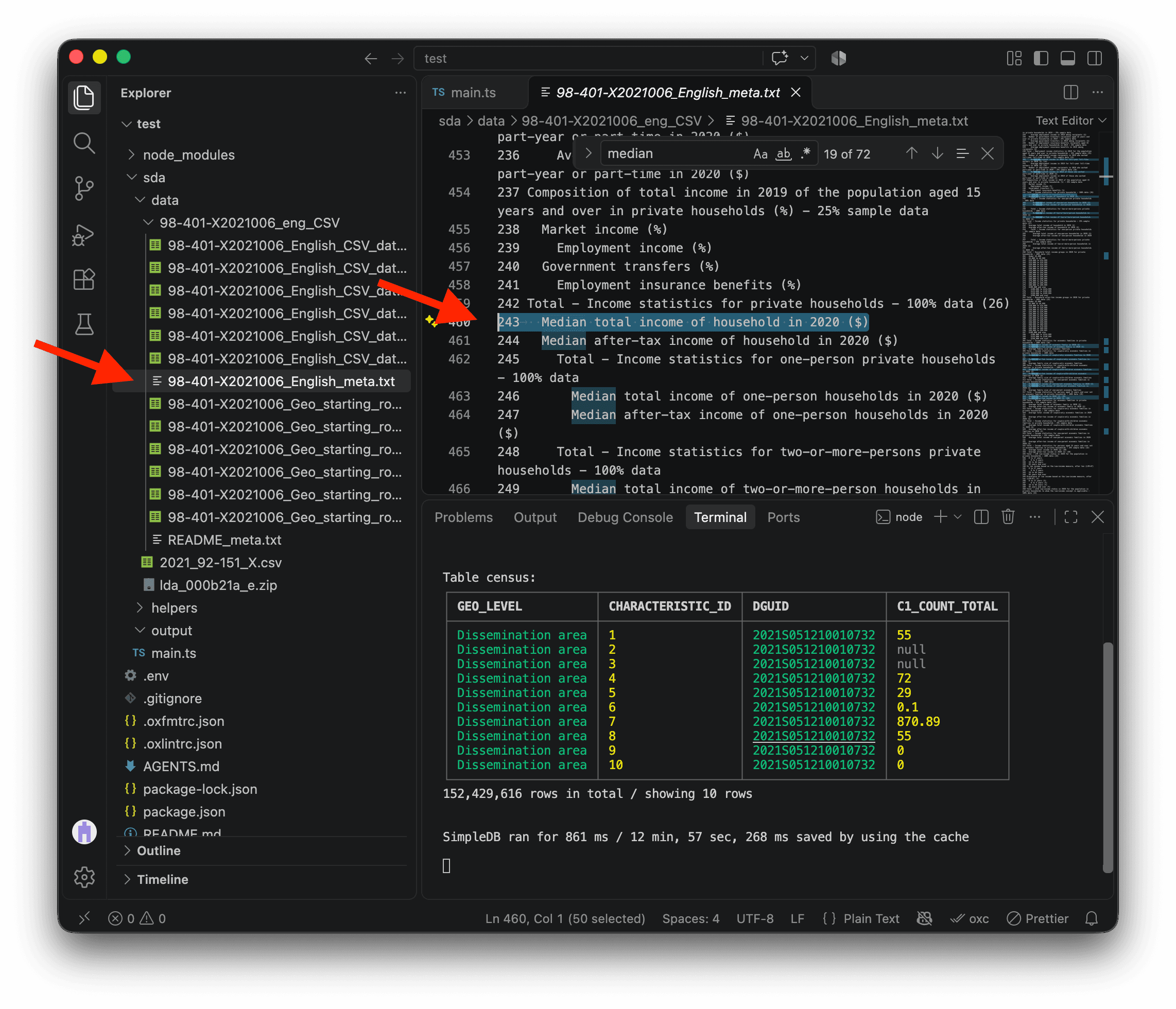
To find the household total income variable, open 98-401-X2021006_English_meta.txt in the Census data folder. This file lists all the Census variables, and it shows that the CHARACTERISTIC_ID for Median total income of household in 2020 ($) is 243.
In the screenshot below, I used search to find it quickly (COMMAND + F on Mac or CTRL + F on Windows).
We can use keepValues to select only rows where CHARACTERISTIC_ID is 243.
⚠️ Make sure to add keepValues after the cache method, as shown below. If you change the code inside cache, SDA will run that entire block again and load the original data. Once the 152 million rows are loaded from the cache, filtering them down to around 57,000 rows is very fast with SDA, so we do not need to cache this step.
import { SimpleDB } from "@nshiab/simple-data-analysis";

const sdb = new SimpleDB({ cacheVerbose: true });

const census = sdb.newTable("census");
await census.cache(() => {
  census.loadData(
    "sda/data/98-401-X2021006_eng_CSV/98-401-X2021006_English_CSV_data_*.csv",
    {
      encoding: "cp1252",
      columns: ["GEO_LEVEL", "CHARACTERISTIC_ID", "DGUID", "C1_COUNT_TOTAL"],
      conditions: `GEO_LEVEL = 'Dissemination area'`,
    },
  );
});
await census
  .keepValues({ CHARACTERISTIC_ID: 243 })
  .log();

await sdb.close();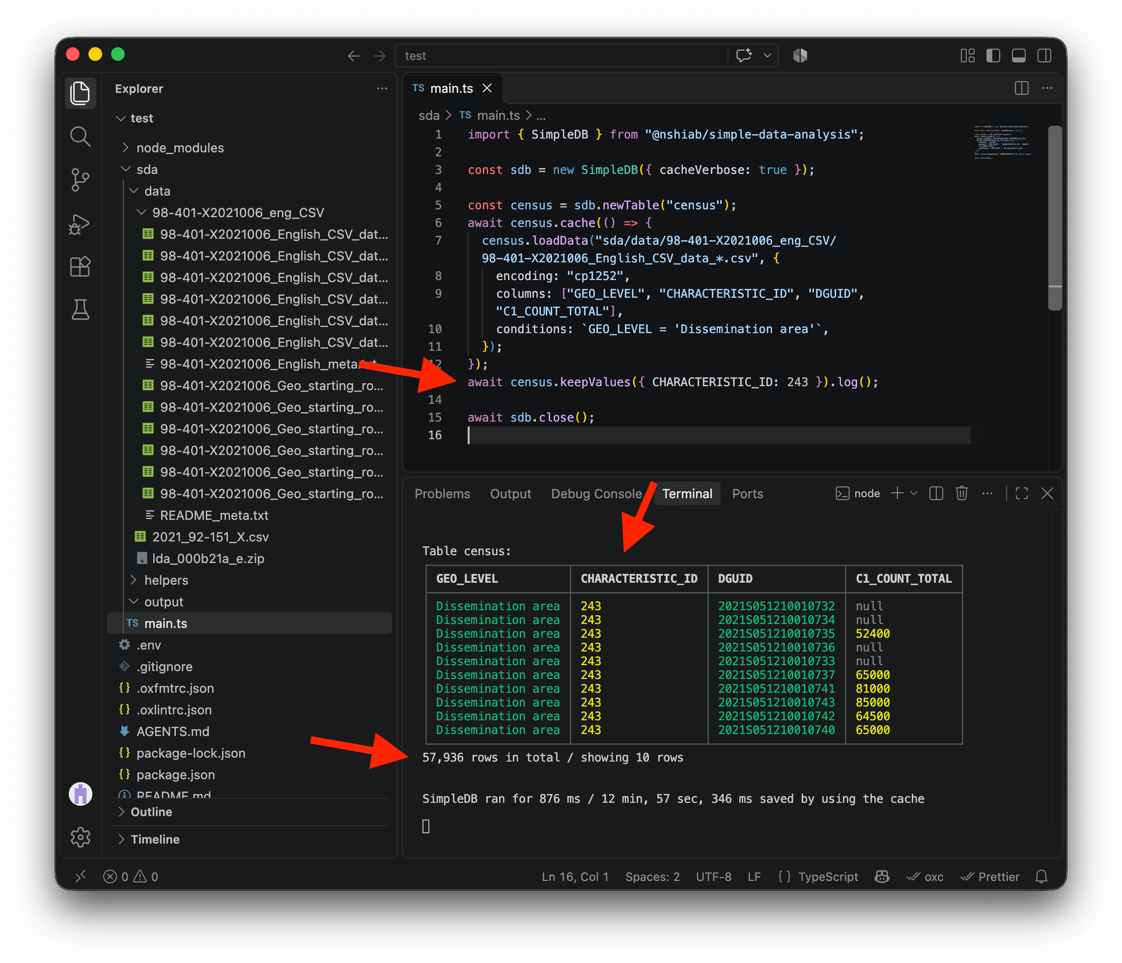
This is looking great! We have the median income for each dissemination area. Now, it would be great to add the metropolitan area names.
The metropolitan areas
To retrieve the metropolitan area names, we’ll use the 2021 Geographic Attribute File we downloaded earlier, stored in 2021_92-151_X.csv. This dataset has many columns, but I went through the documentation for you. We need only two:
DADGUID_ADIDUGD, an ID that matches the dissemination area IDs in the Census dataCMANAME_RMRNOM, the name of the corresponding metropolitan area
The file also uses Windows-1252, so we’ll use the same encoding, columns, and conditions options as before to load only what we need. The condition keeps metropolitan areas, while removeDuplicates gives us unique rows for the next steps. We also use renameColumns so the dissemination area IDs are stored in a column named DGUID in the census table, which stores the Census data, and in the names table, which stores the metropolitan area names.
We will cache this work too. The first run takes a few seconds, but subsequent runs are almost instant.
import { SimpleDB } from "@nshiab/simple-data-analysis";

const sdb = new SimpleDB({ cacheVerbose: true });

const census = sdb.newTable("census");
await census.cache(() => {
  census.loadData(
    "sda/data/98-401-X2021006_eng_CSV/98-401-X2021006_English_CSV_data_*.csv",
    {
      encoding: "cp1252",
      columns: ["GEO_LEVEL", "CHARACTERISTIC_ID", "DGUID", "C1_COUNT_TOTAL"],
      conditions: `GEO_LEVEL = 'Dissemination area'`,
    },
  );
});
await census
  .keepValues({ CHARACTERISTIC_ID: 243 })
  .log();

const names = sdb.newTable("names");
await names.cache(() => {
  names.loadData("sda/data/2021_92-151_X.csv", {
    encoding: "cp1252",
    columns: ["DADGUID_ADIDUGD", "CMANAME_RMRNOM"],
    conditions: `CMATYPE_RMRGENRE = 'B'`,
  })
    .removeDuplicates()
    .renameColumns({
      DADGUID_ADIDUGD: "DGUID",
    });
});
await names.log();

await sdb.close();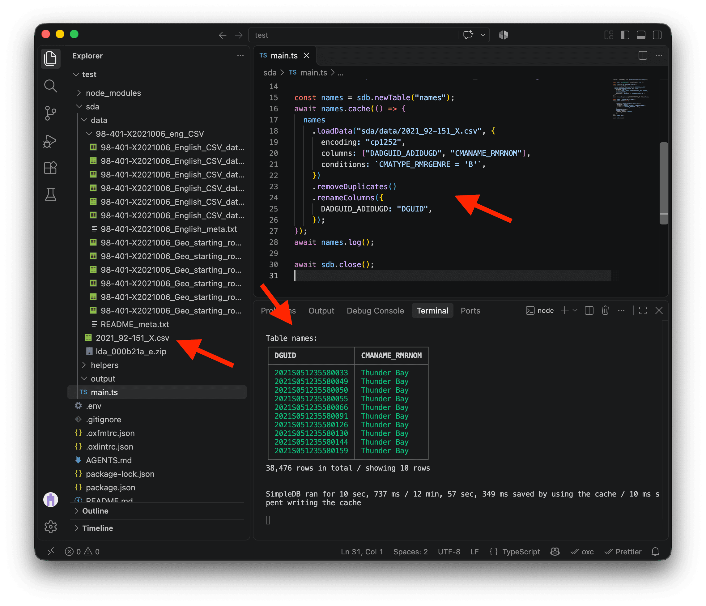
You might have noticed that the names table has around 38,000 rows, while the census table has around 57,000. This is because not every dissemination area belongs to a metropolitan area.
The last step is to join the census table with the names table. The join method automatically finds their shared DGUID column and adds the appropriate metropolitan area name to each matching dissemination area. Now our Census data and metropolitan area names are together in one table! 🎉
import { SimpleDB } from "@nshiab/simple-data-analysis";

const sdb = new SimpleDB({ cacheVerbose: true });

const census = sdb.newTable("census");
await census.cache(() => {
  census.loadData(
    "sda/data/98-401-X2021006_eng_CSV/98-401-X2021006_English_CSV_data_*.csv",
    {
      encoding: "cp1252",
      columns: ["GEO_LEVEL", "CHARACTERISTIC_ID", "DGUID", "C1_COUNT_TOTAL"],
      conditions: `GEO_LEVEL = 'Dissemination area'`,
    },
  );
});
await census
  .keepValues({ CHARACTERISTIC_ID: 243 })
  .log();

const names = sdb.newTable("names");
await names.cache(() => {
  names.loadData("sda/data/2021_92-151_X.csv", {
    encoding: "cp1252",
    columns: ["DADGUID_ADIDUGD", "CMANAME_RMRNOM"],
    conditions: `CMATYPE_RMRGENRE = 'B'`,
  })
    .removeDuplicates()
    .renameColumns({
      DADGUID_ADIDUGD: "DGUID",
    });
});
await names.log();

await census
  .join(names)
  .log();

await sdb.close();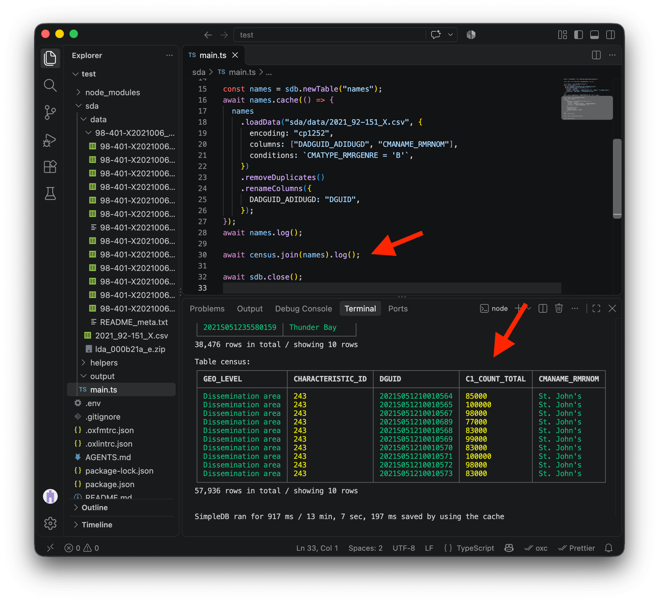
Simplifying the geometries
Since we want to make a map, we need the dissemination areas boundaries. We downloaded them earlier as the zipped file lda_000b21a_e.zip (and I told you not to unzip them 😬).
Statistics Canada provides very detailed geospatial data. But since we only want to draw maps, we don’t need a very high level of detail. A simplified version would be enough and would make our code run faster.
One of my favorite tools to simplify geospatial data is mapshaper.org . Go give them a ⭐ on GitHub if you have an account!
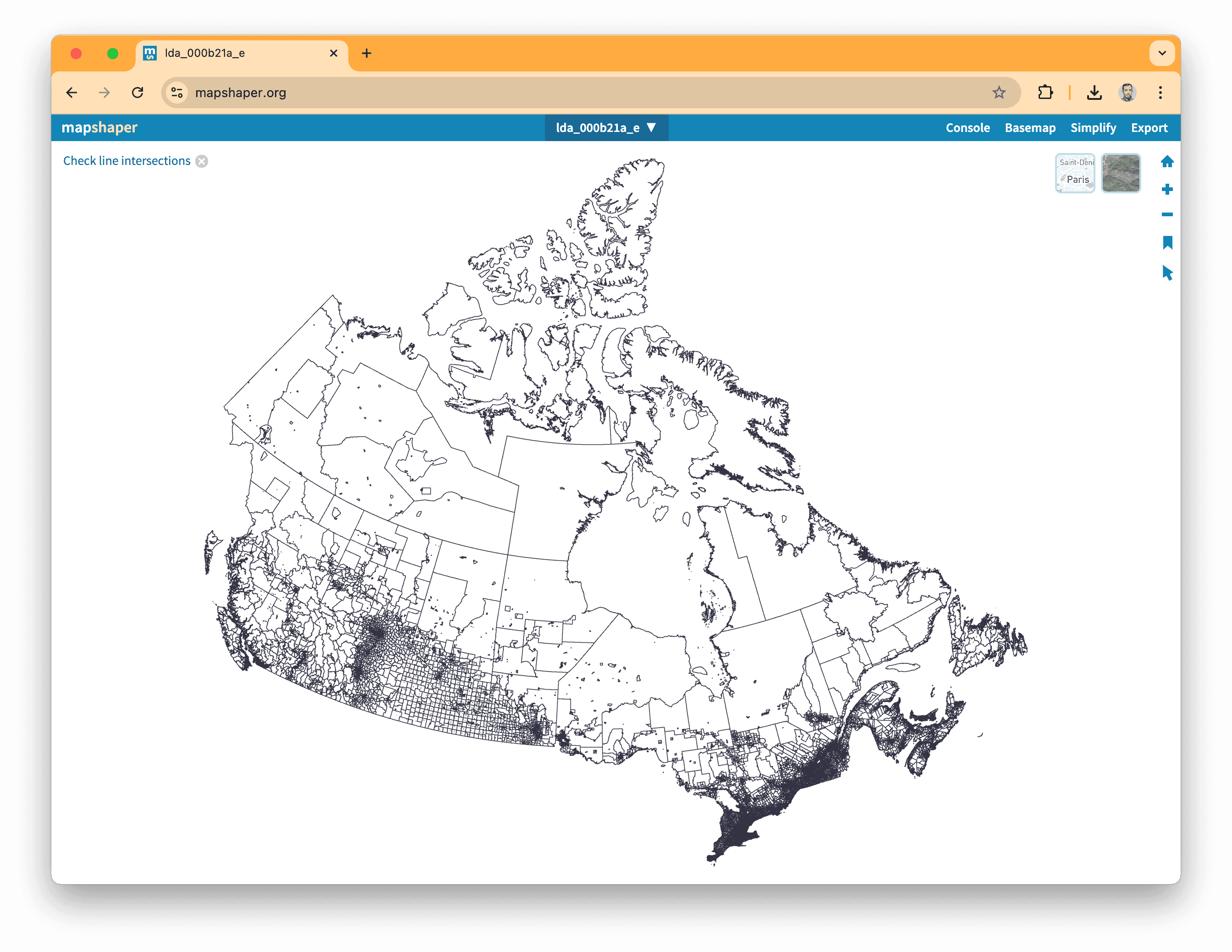
Go on the website and drag-and-drop lda_000b21a_e.zip on the page. Note that you can’t drag-and-drop from VS Code. Do it from your folder using your computer’s Finder or File Explorer.
After a few seconds, you’ll see all the dissemination areas.
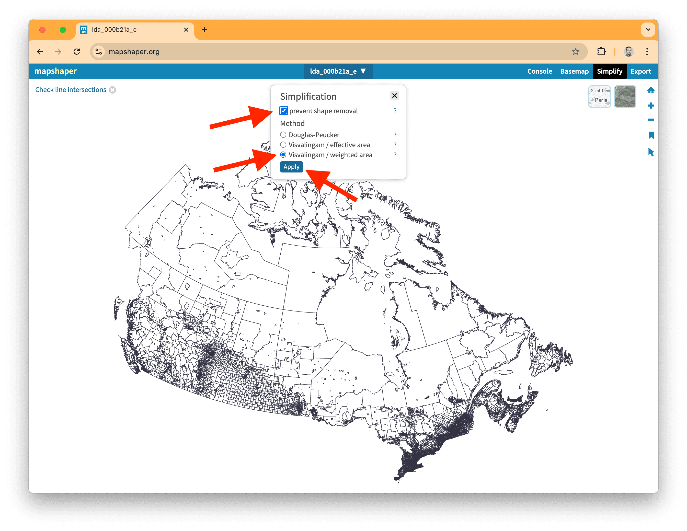
You can now click on Simplify on the top right corner and select the following options:
prevent shape removalVisvalingam / weighted area
Click on Apply!
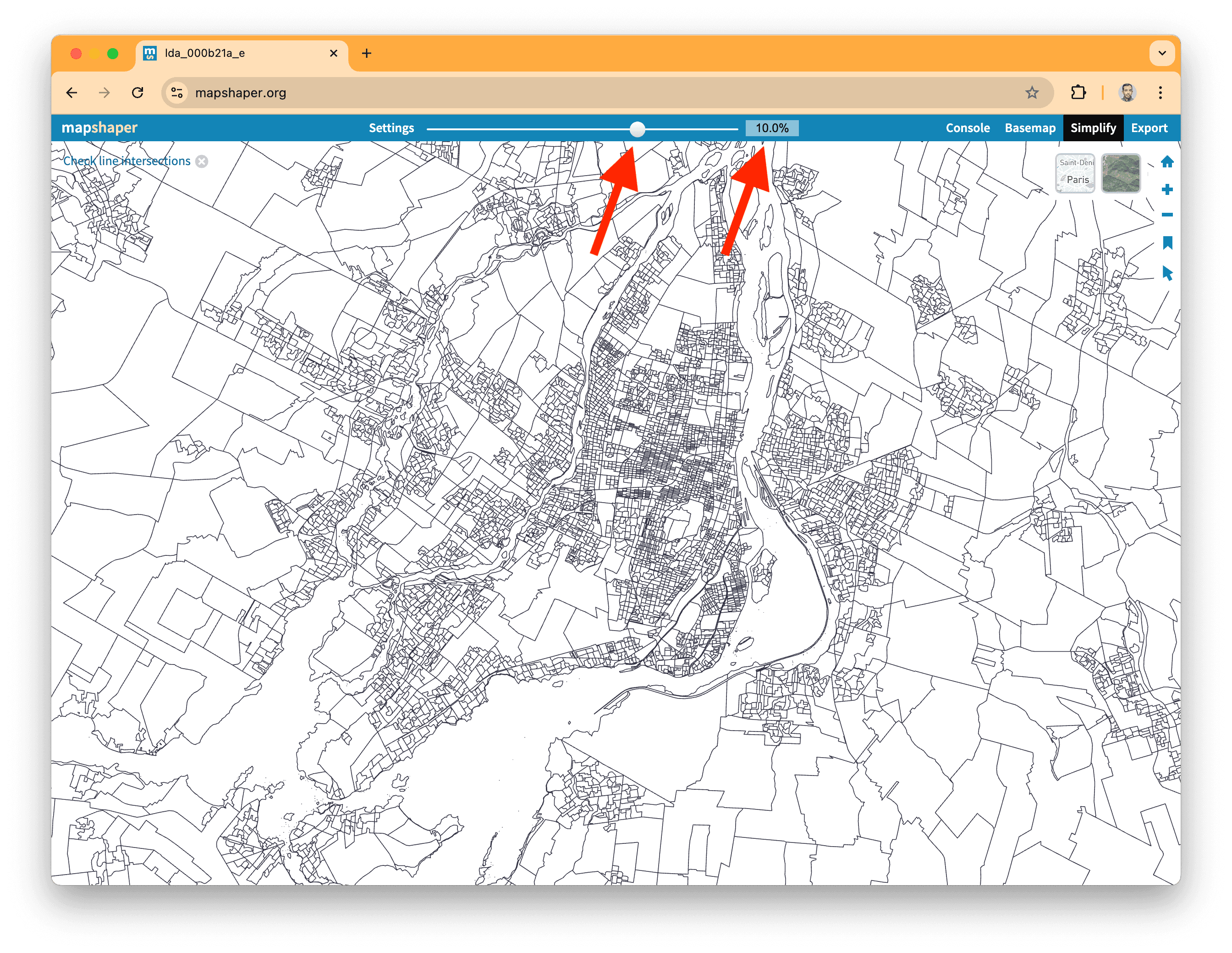
For the next step, I usually zoom in on a high-density area, like Montreal. Then, using the top slider, I aim for a simplification threshold that doesn’t alter the overall shapes.
Here, 10% works pretty well. Note that you can type in the percentage that you want directly too.
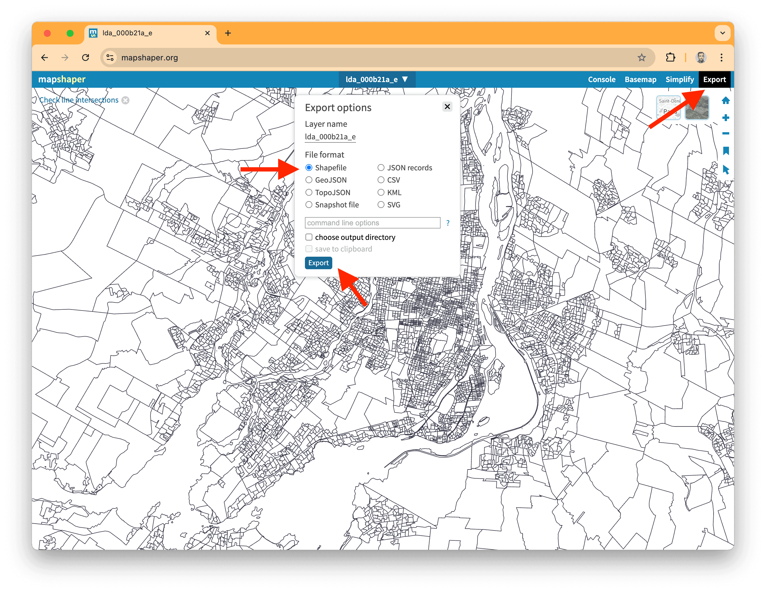
And the next step is to export the simplified data!
Click on the Export button in the top right corner, keep the file format as the original Shapefile, and hit Export.
You can now rename this file lda_000b21a_e.shp.zip (notice I added .shp.zip for the file extension to help SDA understand it’s a shapefile) and move it to your data folder.
Instead of 197 MB, our geospatial data now weighs just 27 MB, which will help speed up our computations and map drawing!
Loading the geometries
To load the geometries, we use loadGeoData instead of loadData. This method stores the boundaries and their coordinates in a spatial geom column. As usual, we use cache to keep everything snappy going forward.
Don’t forget to modify the file extension of your simplified Shapefile to .shp.zip. The shp is important for SDA. Without it, SDA doesn’t recognize the file as a Shapefile and can’t load it correctly.
import { SimpleDB } from "@nshiab/simple-data-analysis";

const sdb = new SimpleDB({ cacheVerbose: true });

const census = sdb.newTable("census");
await census.cache(() => {
  census.loadData(
    "sda/data/98-401-X2021006_eng_CSV/98-401-X2021006_English_CSV_data_*.csv",
    {
      encoding: "cp1252",
      columns: ["GEO_LEVEL", "CHARACTERISTIC_ID", "DGUID", "C1_COUNT_TOTAL"],
      conditions: `GEO_LEVEL = 'Dissemination area'`,
    },
  );
});
await census
  .keepValues({ CHARACTERISTIC_ID: 243 })
  .log();

const names = sdb.newTable("names");
await names.cache(() => {
  names.loadData("sda/data/2021_92-151_X.csv", {
    encoding: "cp1252",
    columns: ["DADGUID_ADIDUGD", "CMANAME_RMRNOM"],
    conditions: `CMATYPE_RMRGENRE = 'B'`,
  })
    .removeDuplicates()
    .renameColumns({
      DADGUID_ADIDUGD: "DGUID",
    });
});
await names.log();

await census
  .join(names)
  .log();

const disseminationAreas = sdb.newTable("disseminationAreas");
await disseminationAreas.cache(() => {
  disseminationAreas.loadGeoData("sda/data/lda_000b21a_e.shp.zip");
});
await disseminationAreas.log();

await sdb.close();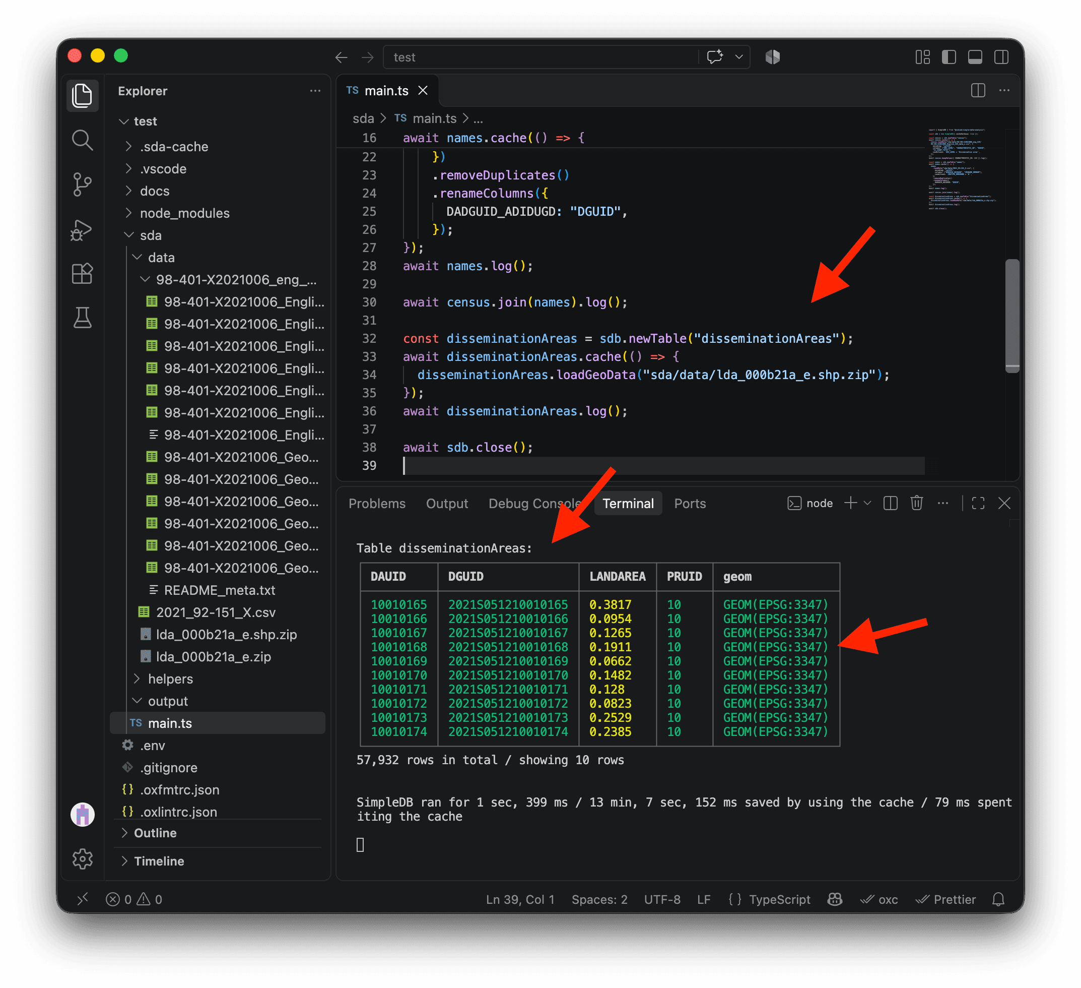
We have no problem loading the geospatial data. We can see the 57,932 dissemination areas as rows with their properties and geometries.
However, the projection is problematic. In the geom column, we can see GEOM(EPSG:3347). This is the Lambert Conformal Conic projection used by Statistics Canada, with coordinates measured in meters. SDA can work with it, but many methods, including those used to draw maps, need EPSG:4326, the widely used projection with latitude and longitude in degrees.
We can use the option toEPSG4326: true to convert the geometries to the right format.
While at it, let’s select only the columns we are interested in:
DGUID, which is the unique ID for dissemination areas. We will use it to join the geometries to the census data.geom, which stores the geometries.
import { SimpleDB } from "@nshiab/simple-data-analysis";

const sdb = new SimpleDB({ cacheVerbose: true });

const census = sdb.newTable("census");
await census.cache(() => {
  census.loadData(
    "sda/data/98-401-X2021006_eng_CSV/98-401-X2021006_English_CSV_data_*.csv",
    {
      encoding: "cp1252",
      columns: ["GEO_LEVEL", "CHARACTERISTIC_ID", "DGUID", "C1_COUNT_TOTAL"],
      conditions: `GEO_LEVEL = 'Dissemination area'`,
    },
  );
});
await census
  .keepValues({ CHARACTERISTIC_ID: 243 })
  .log();

const names = sdb.newTable("names");
await names.cache(() => {
  names.loadData("sda/data/2021_92-151_X.csv", {
    encoding: "cp1252",
    columns: ["DADGUID_ADIDUGD", "CMANAME_RMRNOM"],
    conditions: `CMATYPE_RMRGENRE = 'B'`,
  })
    .removeDuplicates()
    .renameColumns({
      DADGUID_ADIDUGD: "DGUID",
    });
});
await names.log();

await census
  .join(names)
  .log();

const disseminationAreas = sdb.newTable("disseminationAreas");
await disseminationAreas.cache(() => {
  disseminationAreas.loadGeoData("sda/data/lda_000b21a_e.shp.zip", {
    toEPSG4326: true,
    columns: ["DGUID", "geom"],
  });
});
await disseminationAreas.log();

await sdb.close();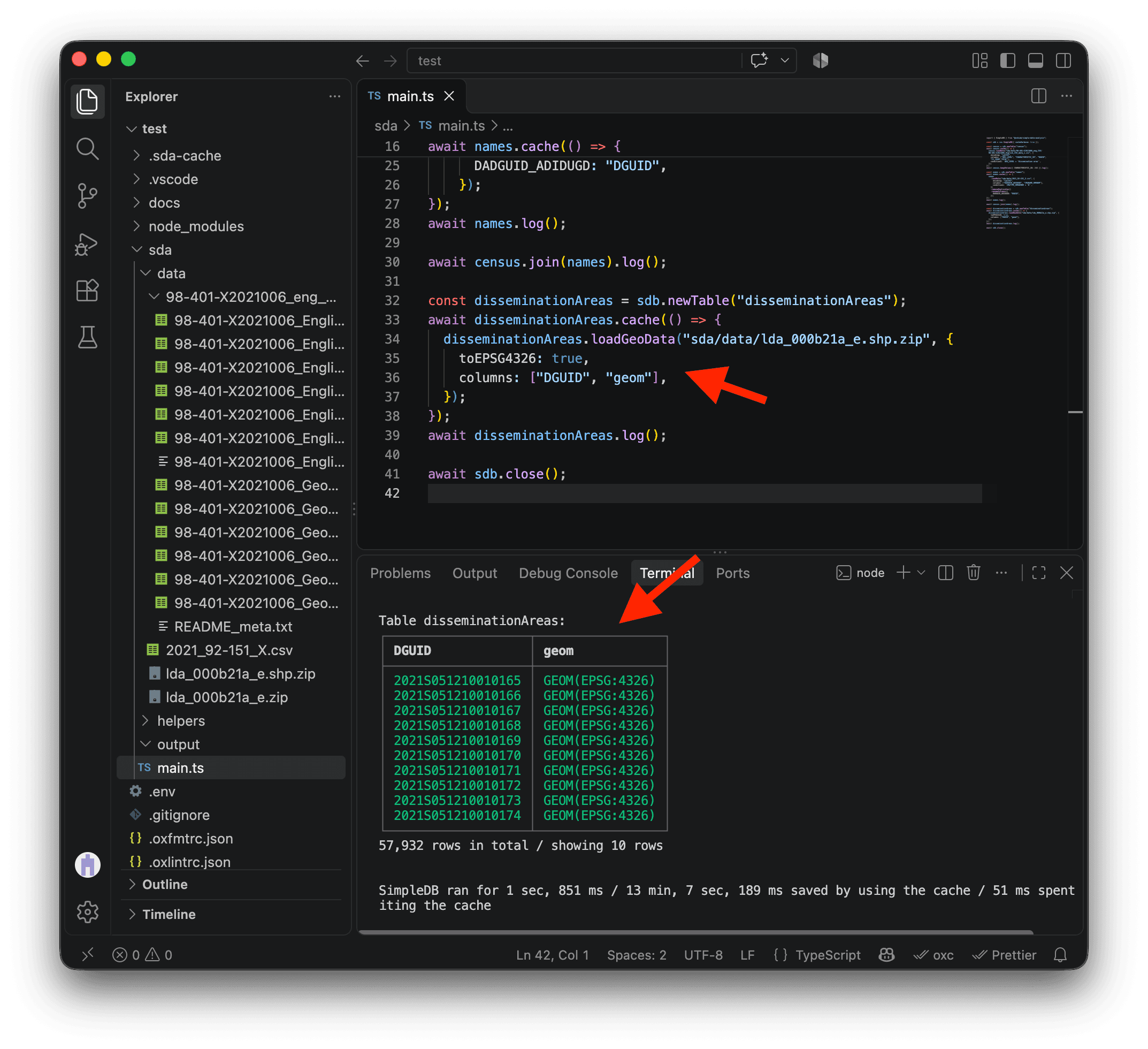
We can now see GEOM(EPSG:4326) in the geom column, confirming that the geometries use the right projection. We also kept DGUID, the unique ID we will use to match these boundaries with the Census dissemination areas.
The last step is to join the dissemination area boundaries with the census data, then call removeMissing(). This keeps only areas with a geometry and a value in C1_COUNT_TOTAL. We now have 37,590 dissemination areas with almost everything we need to make our map! 🗺️
import { SimpleDB } from "@nshiab/simple-data-analysis";

const sdb = new SimpleDB({ cacheVerbose: true });

const census = sdb.newTable("census");
await census.cache(() => {
  census.loadData(
    "sda/data/98-401-X2021006_eng_CSV/98-401-X2021006_English_CSV_data_*.csv",
    {
      encoding: "cp1252",
      columns: ["GEO_LEVEL", "CHARACTERISTIC_ID", "DGUID", "C1_COUNT_TOTAL"],
      conditions: `GEO_LEVEL = 'Dissemination area'`,
    },
  );
});
await census
  .keepValues({ CHARACTERISTIC_ID: 243 })
  .log();

const names = sdb.newTable("names");
await names.cache(() => {
  names.loadData("sda/data/2021_92-151_X.csv", {
    encoding: "cp1252",
    columns: ["DADGUID_ADIDUGD", "CMANAME_RMRNOM"],
    conditions: `CMATYPE_RMRGENRE = 'B'`,
  })
    .removeDuplicates()
    .renameColumns({
      DADGUID_ADIDUGD: "DGUID",
    });
});
await names.log();

await census
  .join(names)
  .log();

const disseminationAreas = sdb.newTable("disseminationAreas");
await disseminationAreas.cache(() => {
  disseminationAreas.loadGeoData("sda/data/lda_000b21a_e.shp.zip", {
    toEPSG4326: true,
    columns: ["DGUID", "geom"],
  });
});
await disseminationAreas
  .join(census)
  .removeMissing()
  .log();

await sdb.close();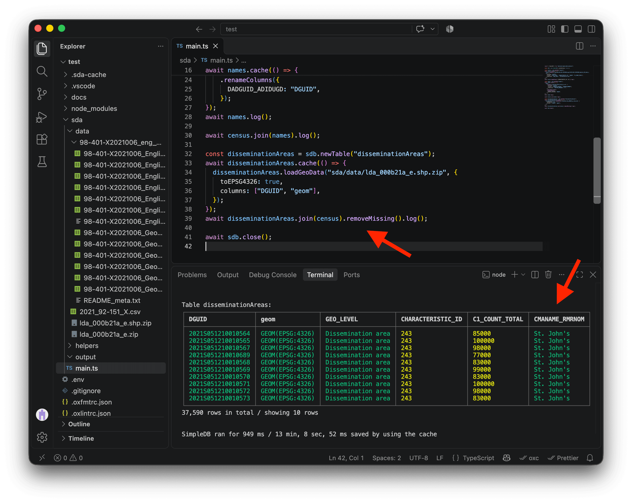
Before we go further, let’s refactor the code we’ve written so far. It builds our dissemination areas table, so let’s move it into a helper function called getDisseminationAreas in the helpers folder. Don’t worry: the cache is clever enough to recognize that the code hasn’t changed, even though it’s in a different file. We’ll keep all the speed benefits of caching! ⚡
We add export default on line 3 so we can import this function elsewhere in our code. We also return disseminationAreas on line 43 so we can work with the table the function creates. Now that we know what each step does, I’ve removed the intermediate .log() calls and kept only the last one to keep the terminal clean.
import { SimpleDB } from "@nshiab/simple-data-analysis";

export default async function getDisseminationAreas(sdb: SimpleDB) {
  const census = sdb.newTable("census");
  await census.cache(() => {
    census.loadData(
      "sda/data/98-401-X2021006_eng_CSV/98-401-X2021006_English_CSV_data_*.csv",
      {
        encoding: "cp1252",
        columns: ["GEO_LEVEL", "CHARACTERISTIC_ID", "DGUID", "C1_COUNT_TOTAL"],
        conditions: `GEO_LEVEL = 'Dissemination area'`,
      },
    );
  });
  census.keepValues({ CHARACTERISTIC_ID: 243 });

  const names = sdb.newTable("names");
  await names.cache(() => {
    names.loadData("sda/data/2021_92-151_X.csv", {
      encoding: "cp1252",
      columns: ["DADGUID_ADIDUGD", "CMANAME_RMRNOM"],
      conditions: `CMATYPE_RMRGENRE = 'B'`,
    })
      .removeDuplicates()
      .renameColumns({
        DADGUID_ADIDUGD: "DGUID",
      });
  });
  census.join(names);

  const disseminationAreas = sdb.newTable("disseminationAreas");
  await disseminationAreas.cache(() => {
    disseminationAreas.loadGeoData("sda/data/lda_000b21a_e.shp.zip", {
      toEPSG4326: true,
      columns: ["DGUID", "geom"],
    });
  });
  await disseminationAreas
    .join(census)
    .removeMissing()
    .log();

  return disseminationAreas;
}
Now we can import and call getDisseminationAreas in main.ts, and store the result in the disseminationAreas constant.
import { SimpleDB } from "@nshiab/simple-data-analysis";
import getDisseminationAreas from "./helpers/getDisseminationAreas.ts";

const sdb = new SimpleDB({ cacheVerbose: true });

const disseminationAreas = await getDisseminationAreas(sdb);

await sdb.close();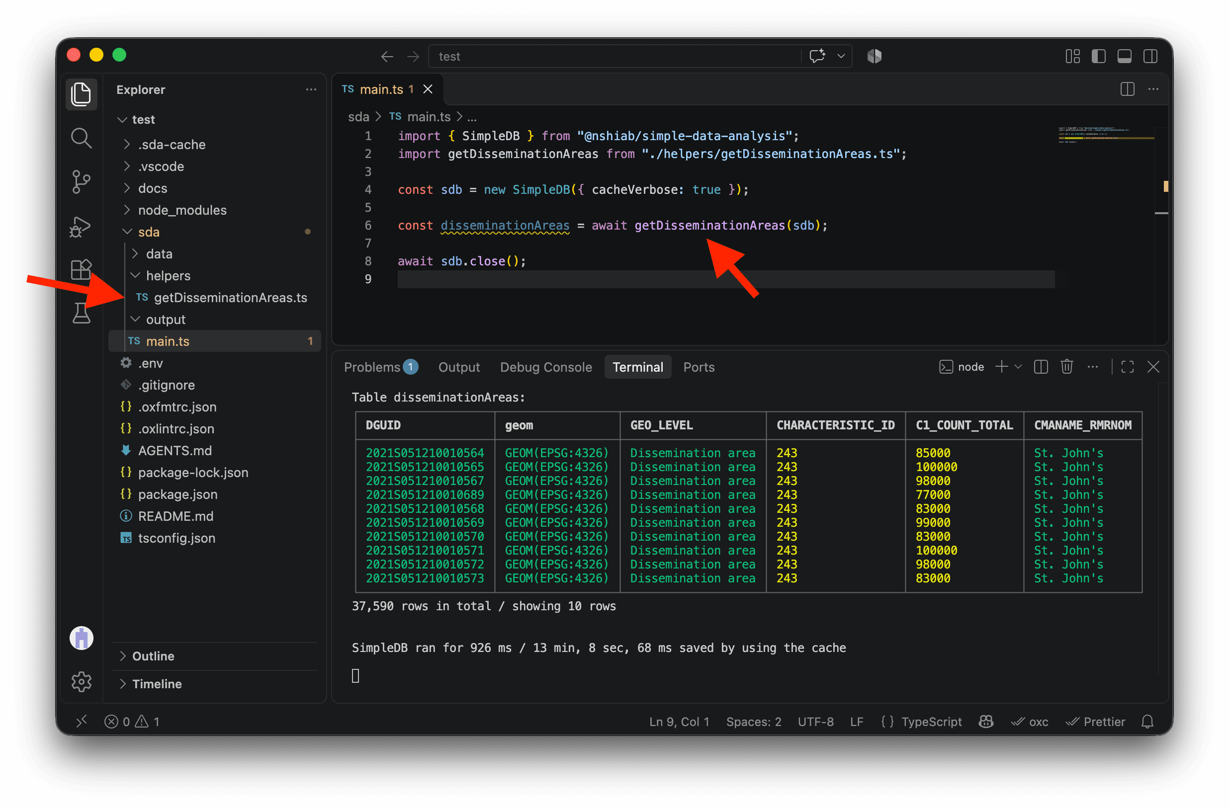
VS Code underlines disseminationAreas in yellow on line 6 because we’re not using this variable in the current code. If you scroll up in the terminal, you’ll see the same warning. Warnings let the code run, while errors stop it. This warning helps us spot variables we can remove to keep our analysis code easy to follow. We’ll use disseminationAreas in the next section.
Answering the question
Now that we have the Census data and the dissemination area geometries together, we can answer our question:
- For each Canadian metropolitan area, which dissemination areas have household incomes above or below the median?
Comparing incomes with the median
For each dissemination area, we want to know how far its median household income is above or below the median across dissemination areas in its metropolitan area. The percentChange method calculates that percentage difference directly. Create addMedianVariation.ts in the helpers folder.
"C1_COUNT_TOTAL"contains the median household income for each dissemination area.{ stat: "median", by: "CMANAME_RMRNOM" }uses the median of those values within each metropolitan area as the reference."percVar"names the new column that stores the result.base: 100expresses the difference as a percentage, anddecimals: 0rounds it to the nearest whole number.
import type { SimpleTable } from "@nshiab/simple-data-analysis";

export default async function addMedianVariation(disseminationAreas: SimpleTable) {
  await disseminationAreas
    .percentChange("C1_COUNT_TOTAL", { stat: "median", by: "CMANAME_RMRNOM" }, "percVar", {
      base: 100,
      decimals: 0,
    })
    .log();
}
Now we can import addMedianVariation in main.ts and call it with our disseminationAreas table.
import { SimpleDB } from "@nshiab/simple-data-analysis";
import getDisseminationAreas from "./helpers/getDisseminationAreas.ts";
import addMedianVariation from "./helpers/addMedianVariation.ts";

const sdb = new SimpleDB({ cacheVerbose: true });

const disseminationAreas = await getDisseminationAreas(sdb);
await addMedianVariation(disseminationAreas);

await sdb.close();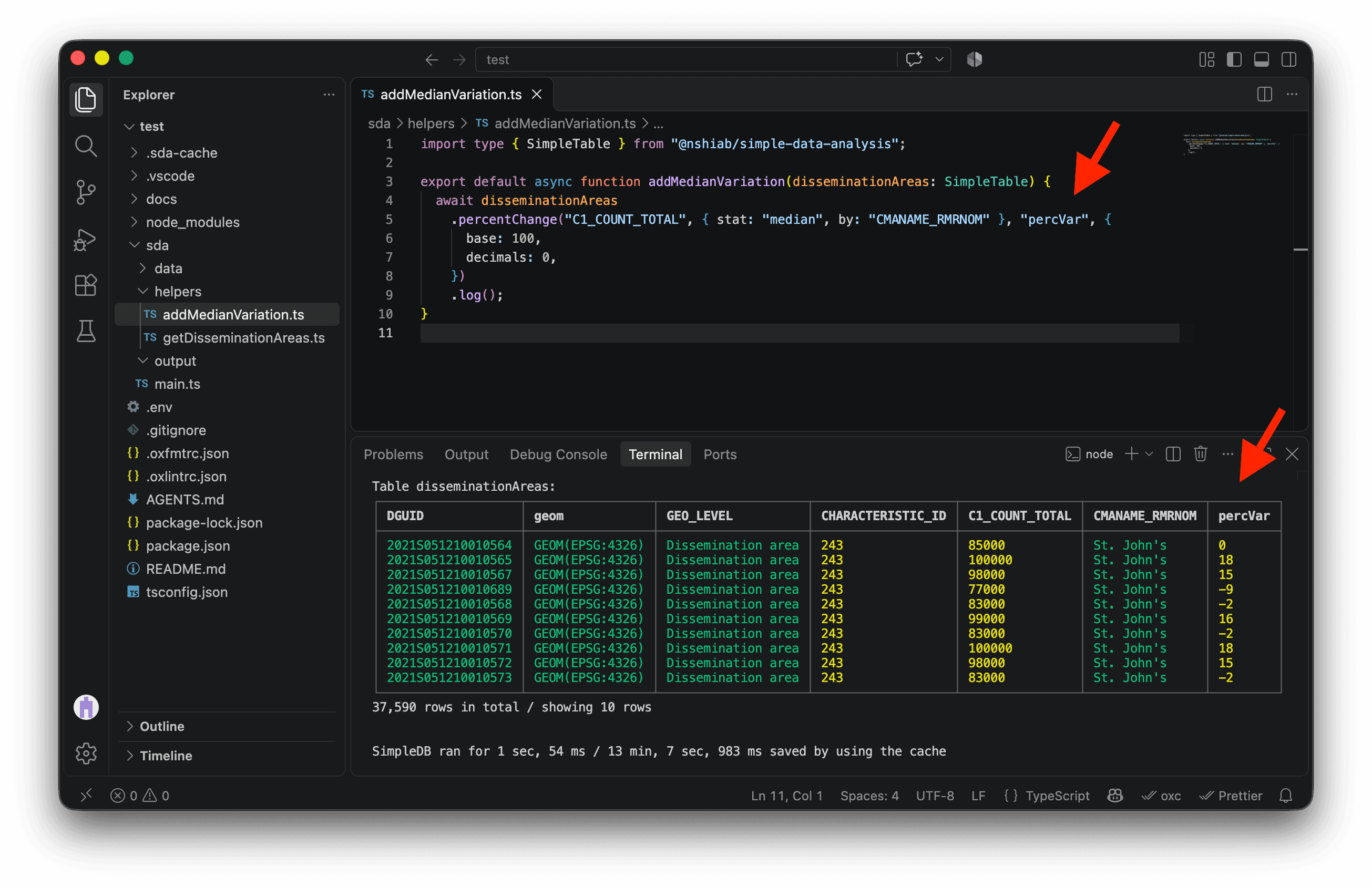
We finally have the answer to our question! For each of the 37,590 dissemination areas in metropolitan areas, percVar shows whether its median household income is above or below the median across dissemination areas in its metropolitan area, and by what percentage. Now we’re ready to make one map per metropolitan area! 🚀
Making maps
To keep our code organized and to stay mentally sane, let’s create a new file, visualizeData.ts, in helpers. This is where we’ll put the code that makes our maps.
The new function takes our disseminationAreas table as a SimpleTable. For now, it just logs a message in the terminal.
import type { SimpleTable } from "@nshiab/simple-data-analysis";

export default async function visualizeData(
  disseminationAreas: SimpleTable,
) {
  console.log("\nVisualizing dissemination areas data...");
}
Now let’s import and call visualizeData in main.ts.
import { SimpleDB } from "@nshiab/simple-data-analysis";
import getDisseminationAreas from "./helpers/getDisseminationAreas.ts";
import addMedianVariation from "./helpers/addMedianVariation.ts";
import visualizeData from "./helpers/visualizeData.ts";

const sdb = new SimpleDB({ cacheVerbose: true });

const disseminationAreas = await getDisseminationAreas(sdb);
await addMedianVariation(disseminationAreas);
await visualizeData(disseminationAreas);

await sdb.close();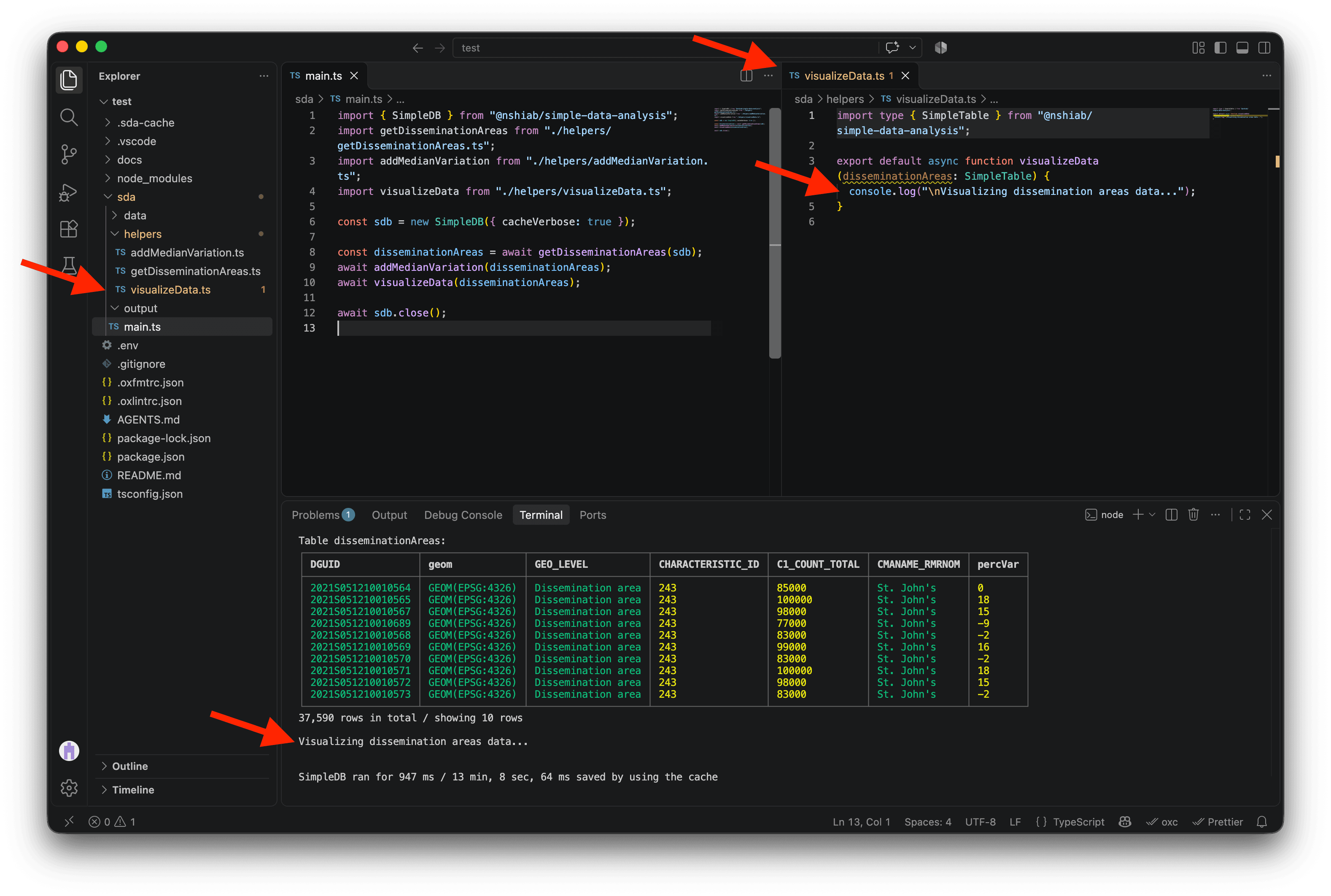
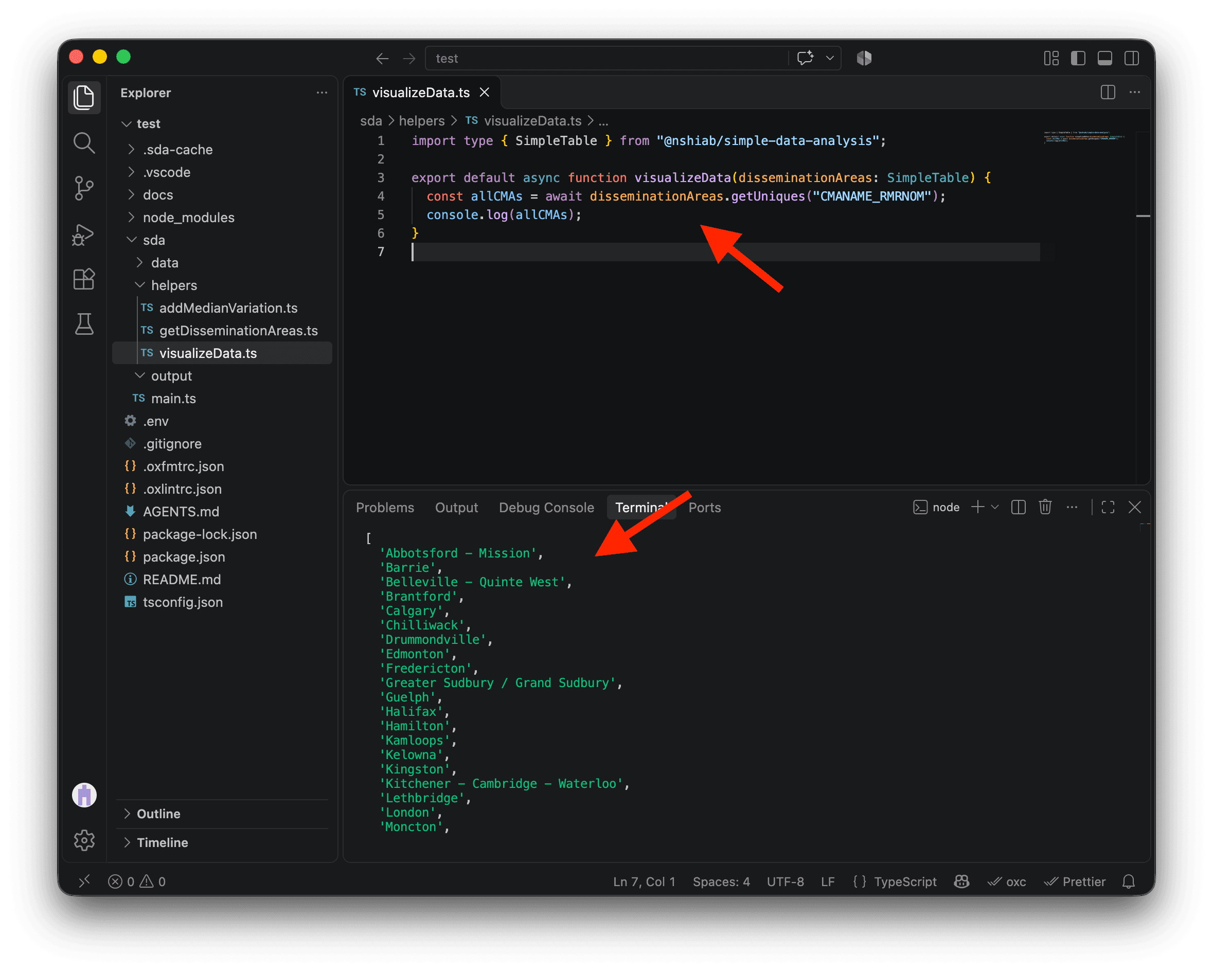
We want to draw a map for each metropolitan area. First, let’s retrieve all the unique metropolitan area names in our data with getUniques. Logging allCMAs shows the list we’ll use to loop over the areas and draw a map for each one.
import type { SimpleTable } from "@nshiab/simple-data-analysis";

export default async function visualizeData(
  disseminationAreas: SimpleTable,
) {
  const allCMAs = await disseminationAreas.getUniques("CMANAME_RMRNOM");
  console.log(allCMAs);
}
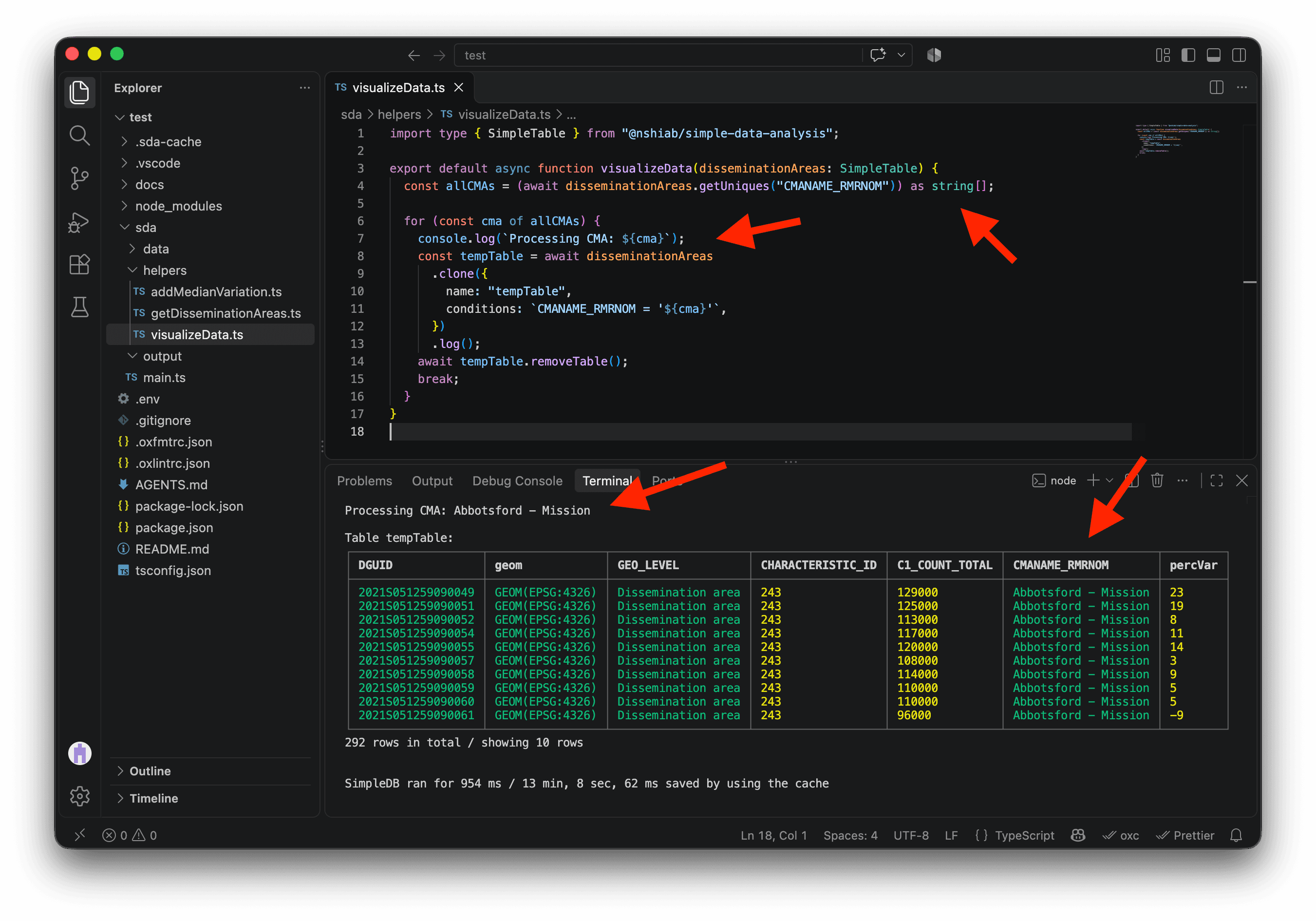
Now we can loop through the metropolitan areas one by one. In the code below, we log the CMA we’re processing. Then we clone disseminationAreas into a temporary table, using conditions to keep only rows for that CMA, and log the result.
At the end of each iteration, we remove tempTable so the next one starts fresh. For now, break on line 17 stops after the first CMA. Once the map works for one area, we’ll remove it and process them all.
import type { SimpleTable } from "@nshiab/simple-data-analysis";

export default async function visualizeData(
  disseminationAreas: SimpleTable,
) {
  const allCMAs = (await disseminationAreas.getUniques("CMANAME_RMRNOM")) as string[];

  for (const cma of allCMAs) {
    console.log(`Processing CMA: ${cma}`);
    const tempTable = await disseminationAreas
      .clone({
        name: "tempTable",
        conditions: `CMANAME_RMRNOM = '${cma}'`,
      })
      .log();
    await tempTable.removeTable();
    break;
  }
}We give TypeScript a little help on line 6 by adding as string[]. We saw in the terminal that getUniques gives us a list of CMA names, so we tell TypeScript to treat them as strings. That lets us use cma in the strings on lines 9 and 13 without a warning.
As we can see, the first metropolitan area we’re processing is Abbotsford–Mission. The temporary table contains just 292 rows, all from that metropolitan area.
We can now draw our first map. When we ran setup-data-project, it automatically installed Plot . This powerful data visualization library works well with SDA and will help us draw the map.
Using writeMap with Plot’s plot and geo, we draw the dissemination area boundaries. Setting fill to percVar colors each area according to its percentage variation from the metropolitan area’s median.
import type { SimpleTable } from "@nshiab/simple-data-analysis";
import { geo, plot } from "@observablehq/plot";

export default async function visualizeData(
  disseminationAreas: SimpleTable,
) {
  const allCMAs = (await disseminationAreas.getUniques("CMANAME_RMRNOM")) as string[];

  for (const cma of allCMAs) {
    console.log(`Processing CMA: ${cma}`);

    const tempTable = await disseminationAreas
      .clone({
        name: "tempTable",
        conditions: `CMANAME_RMRNOM = '${cma}'`,
      })
      .writeMap(
        (geoData) =>
          plot({
            marks: [
              geo(geoData, {
                fill: "percVar",
              }),
            ],
          }),
        `./sda/output/${cma}.png`,
      );

    await tempTable.removeTable();
    break;
  }
}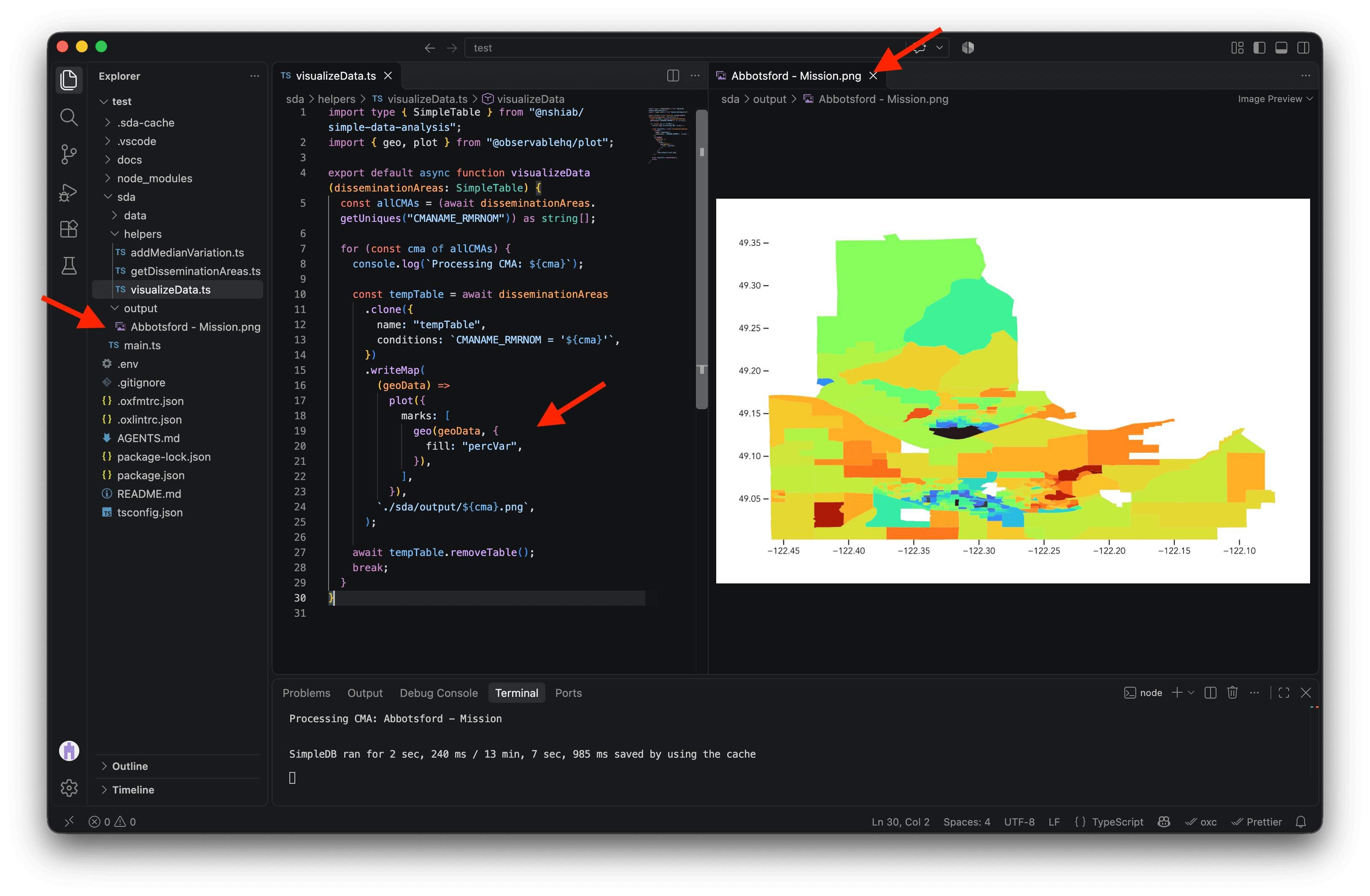
It’s ugly, but it works!
We can now add a title, subtitle, caption, diverging color scale, and map projection. Some dissemination areas have incomes 200%, 300%, or even 400% above their metropolitan area’s median, which can make smaller differences hard to see. Setting the color domain to [-100, 100] keeps the scale focused; values above +100% use its most saturated positive color. For more on these customizations, check the Visualizing data lesson.
import type { SimpleTable } from "@nshiab/simple-data-analysis";
import { geo, plot } from "@observablehq/plot";

export default async function visualizeData(
  disseminationAreas: SimpleTable,
) {
  const allCMAs = (await disseminationAreas.getUniques("CMANAME_RMRNOM")) as string[];

  for (const cma of allCMAs) {
    console.log(`Processing CMA: ${cma}`);

    const tempTable = await disseminationAreas
      .clone({
        name: "tempTable",
        conditions: `CMANAME_RMRNOM = '${cma}'`,
      })
      .writeMap(
        (geoData) =>
          plot({
            title: cma,
            subtitle:
              "Variation from the median household total income at the dissemination area level.",
            caption: "2021 Census, Statistics Canada",
            projection: {
              type: "mercator",
              domain: geoData,
            },
            color: {
              legend: true,
              type: "diverging",
              domain: [-100, 100],
              ticks: 5,
              tickFormat: (d) => {
                if (d > 0) {
                  return `+${d}%`;
                }
                return `${d}%`;
              },
              label: null,
            },
            marks: [
              geo(geoData, {
                fill: "percVar",
              }),
            ],
          }),
        `./sda/output/${cma}.png`,
      );

    await tempTable.removeTable();
    break;
  }
}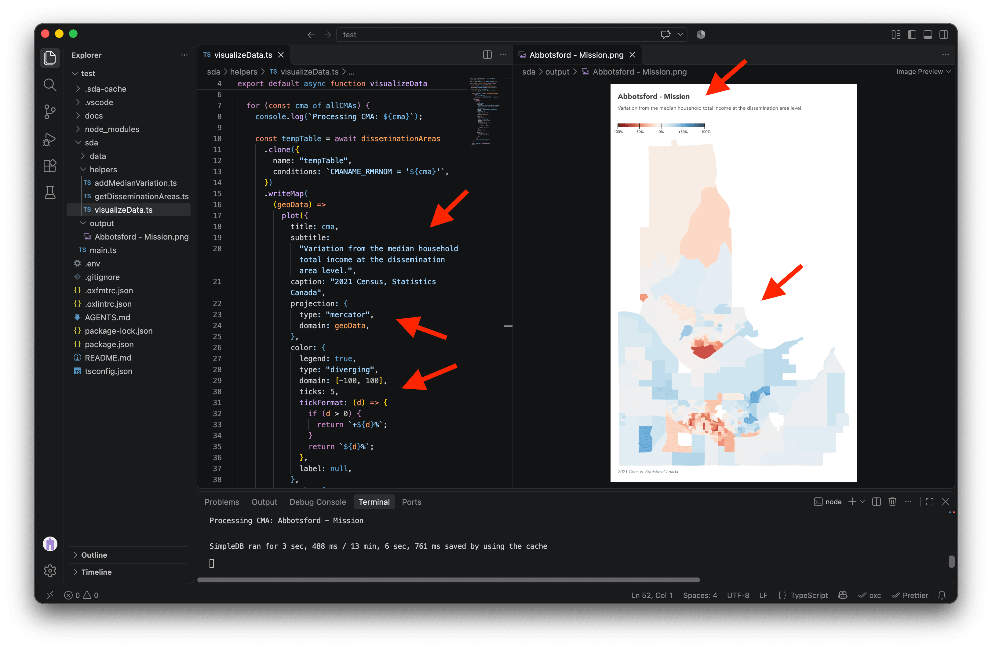
This is looking much better! 💅
One last touch: let’s add an outline around the metropolitan area. In the new code below, we clone tempTable inside the loop to create an outline table. Calling aggregateGeo("union") merges its dissemination area geometries into one polygon, leaving one row with the metropolitan area’s boundary.
We then use insertTables to add that row to tempTable. The unifyColumns option is needed because outline has only a geom column, while tempTable also has the Census columns. In writeMap, a second geo mark selects the feature whose percVar is null (our outline) and draws it with a partly transparent black stroke.
We also remove the outline table after writing the map, so each loop iteration can create a fresh one.
If this feels like a lot, try the Visualizing data lesson again before moving on.
import type { SimpleTable } from "@nshiab/simple-data-analysis";
import { geo, plot } from "@observablehq/plot";

export default async function visualizeData(
  disseminationAreas: SimpleTable,
) {
  const allCMAs = (await disseminationAreas.getUniques("CMANAME_RMRNOM")) as string[];

  for (const cma of allCMAs) {
    console.log(`Processing CMA: ${cma}`);

    const tempTable = await disseminationAreas
      .clone({
        name: "tempTable",
        conditions: `CMANAME_RMRNOM = '${cma}'`,
      });

    const outline = tempTable
      .clone("outline")
      .aggregateGeo("union");

    tempTable.insertTables(outline, { unifyColumns: true });

    await tempTable.writeMap(
      (geoData) =>
        plot({
          title: cma,
          subtitle:
            "Variation from the median household total income at the dissemination area level.",
          caption: "2021 Census, Statistics Canada",
          projection: {
            type: "mercator",
            domain: geoData,
          },
          color: {
            legend: true,
            type: "diverging",
            domain: [-100, 100],
            ticks: 5,
            tickFormat: (d) => {
              if (d > 0) {
                return `+${d}%`;
              }
              return `${d}%`;
            },
            label: null,
          },
          marks: [
            geo(geoData, {
              fill: "percVar",
            }),
            geo(geoData.features.filter((d) => d.properties.percVar === null), {
              stroke: "black",
              strokeOpacity: 0.5,
            }),
          ],
        }),
      `./sda/output/${cma}.png`,
    );

    await outline.removeTable();
    await tempTable.removeTable();
    break;
  }
}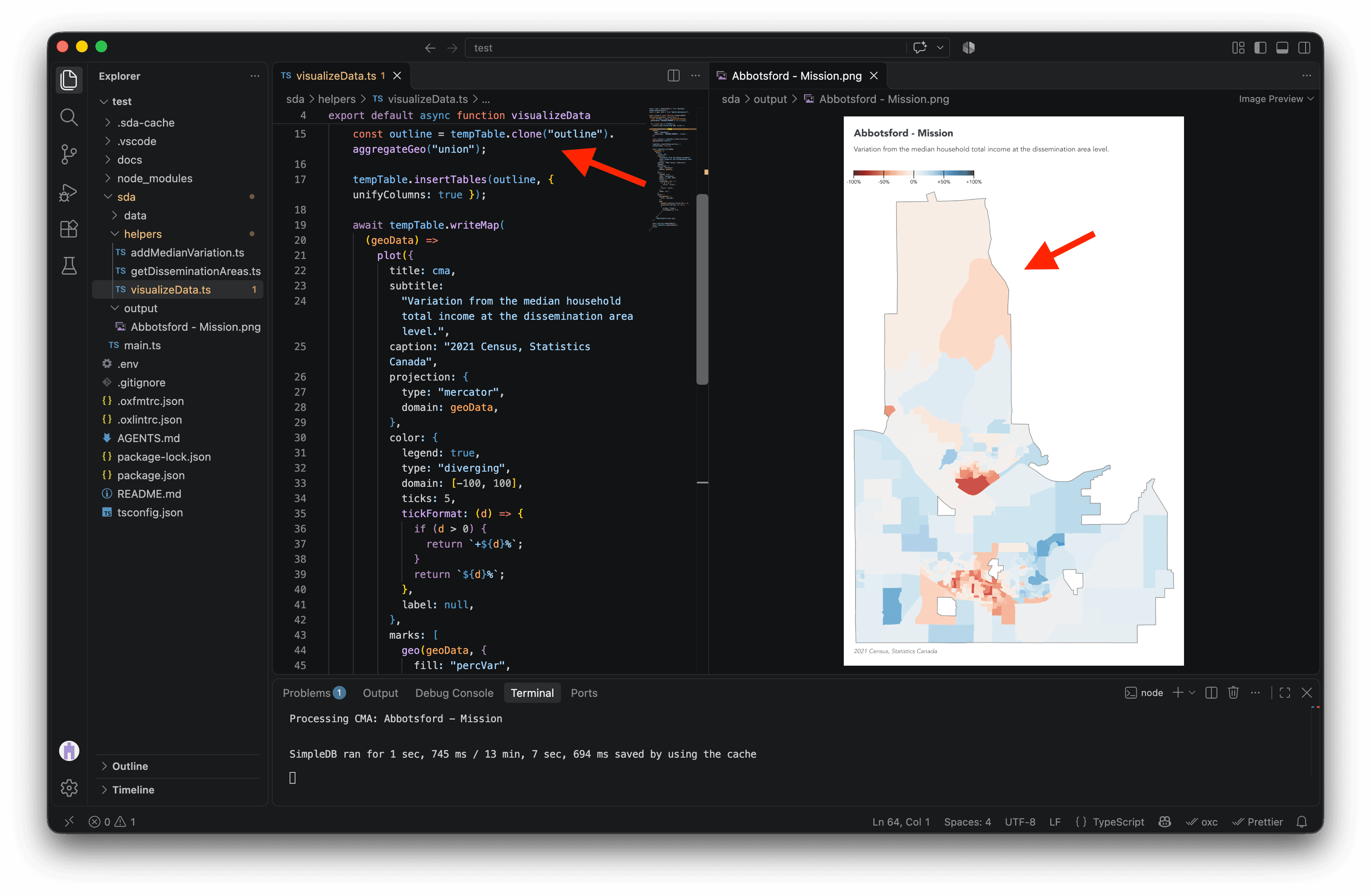
The difference is subtle, but the outline helps us see holes in the metropolitan area geometry. It also makes the boundary visible where dissemination areas near the edge are white or almost white.
We’re almost ready to remove break and make maps for every metropolitan area. But first, we need to clean the CMA name used in the output path. A name like Greater Sudbury / Grand Sudbury contains /, which would create an unwanted folder in ./sda/output/${cma}.png instead of a single image file.
Second, we need to escape apostrophes in CMA names such as St. John's. Because the SQL condition encloses the name in single quotes, any apostrophe inside it must be doubled.
In the code below, we use replaceAll for both fixes. We also remove break so the loop can create a map for every metropolitan area.
import type { SimpleTable } from "@nshiab/simple-data-analysis";
import { geo, plot } from "@observablehq/plot";

export default async function visualizeData(
  disseminationAreas: SimpleTable,
) {
  const allCMAs = (await disseminationAreas.getUniques("CMANAME_RMRNOM")) as string[];

  for (const cma of allCMAs) {
    console.log(`Processing CMA: ${cma}`);

    const tempTable = disseminationAreas
      .clone({
        name: "tempTable",
        conditions: `CMANAME_RMRNOM = '${cma.replaceAll("'", "''")}'`,
      });

    const outline = tempTable
      .clone("outline")
      .aggregateGeo("union");

    tempTable.insertTables(outline, { unifyColumns: true });

    await tempTable.writeMap(
      (geoData) =>
        plot({
          title: cma,
          subtitle:
            "Variation from the median household total income at the dissemination area level.",
          caption: "2021 Census, Statistics Canada",
          projection: {
            type: "mercator",
            domain: geoData,
          },
          color: {
            legend: true,
            type: "diverging",
            domain: [-100, 100],
            ticks: 5,
            tickFormat: (d) => {
              if (d > 0) {
                return `+${d}%`;
              }
              return `${d}%`;
            },
            label: null,
          },
          marks: [
            geo(geoData, {
              fill: "percVar",
            }),
            geo(geoData.features.filter((d) => d.properties.percVar === null), {
              stroke: "black",
              strokeOpacity: 0.5,
            }),
          ],
        }),
      `./sda/output/${cma.replaceAll("/", "_")}.png`,
    );

    await outline.removeTable();
    await tempTable.removeTable();
  }
}
However, this code processes the first few metropolitan areas, then fails on Calgary. The error suggests that some input geometries are invalid. 🤔
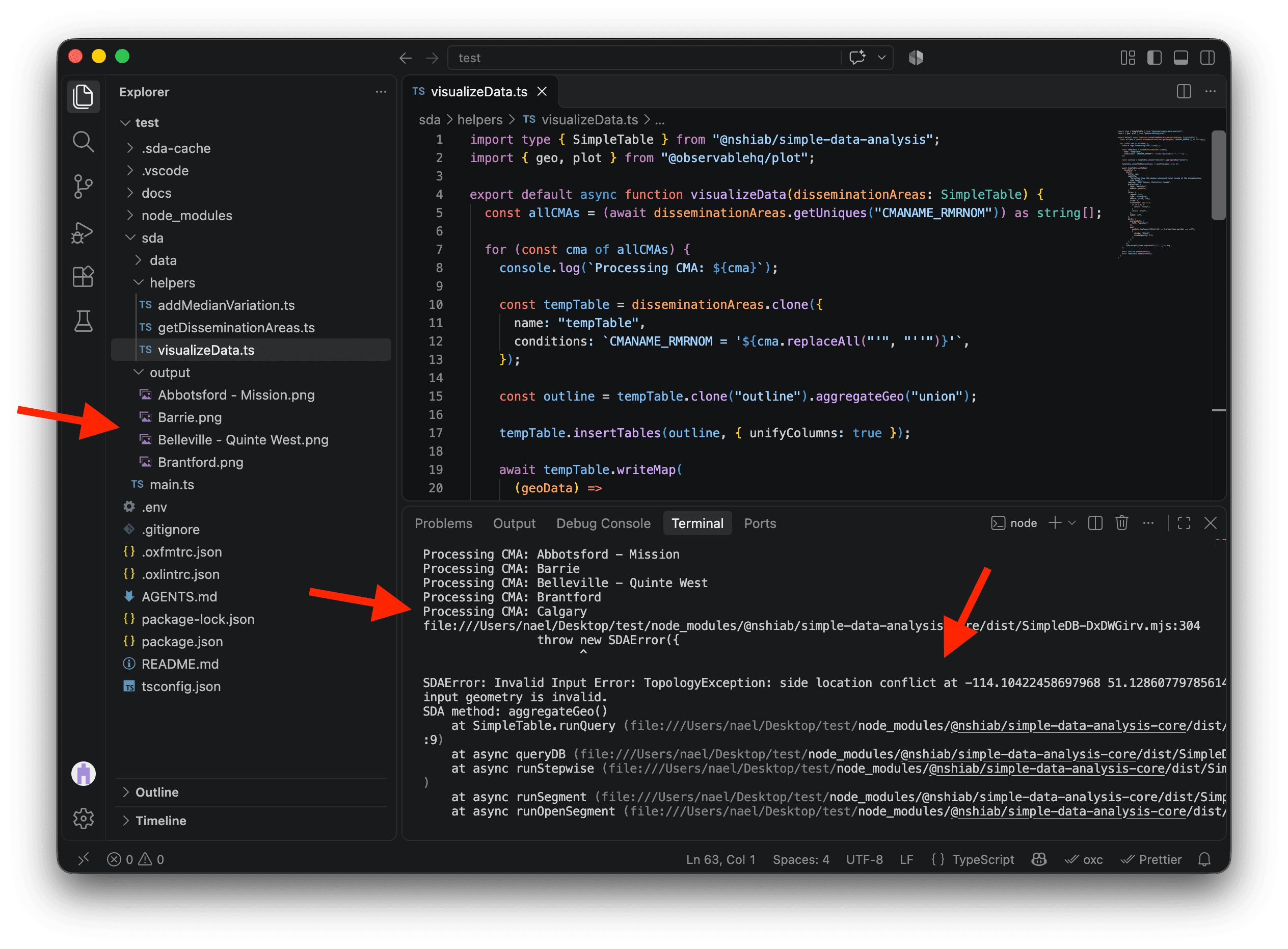
Luckily, SDA makes invalid geometries easy to fix with fixGeo(). We load the dissemination area boundaries in getDisseminationAreas, so we can chain it after loadGeoData() inside cache(). SDA will repair the geometries as they load and cache the fixed result for later runs.
import { SimpleDB } from "@nshiab/simple-data-analysis";

export default async function getDisseminationAreas(sdb: SimpleDB) {
  const census = sdb.newTable("census");
  await census.cache(() => {
    census.loadData(
      "sda/data/98-401-X2021006_eng_CSV/98-401-X2021006_English_CSV_data_*.csv",
      {
        encoding: "cp1252",
        columns: ["GEO_LEVEL", "CHARACTERISTIC_ID", "DGUID", "C1_COUNT_TOTAL"],
        conditions: `GEO_LEVEL = 'Dissemination area'`,
      },
    );
  });
  census.keepValues({ CHARACTERISTIC_ID: 243 });

  const names = sdb.newTable("names");
  await names.cache(() => {
    names.loadData("sda/data/2021_92-151_X.csv", {
      encoding: "cp1252",
      columns: ["DADGUID_ADIDUGD", "CMANAME_RMRNOM"],
      conditions: `CMATYPE_RMRGENRE = 'B'`,
    })
      .removeDuplicates()
      .renameColumns({
        DADGUID_ADIDUGD: "DGUID",
      });
  });
  census.join(names);

  const disseminationAreas = sdb.newTable("disseminationAreas");
  await disseminationAreas.cache(() => {
    disseminationAreas
      .loadGeoData("sda/data/lda_000b21a_e.shp.zip", {
        toEPSG4326: true,
        columns: ["DGUID", "geom"],
      })
      .fixGeo();
  });
  await disseminationAreas
    .join(census)
    .removeMissing()
    .log();

  return disseminationAreas;
}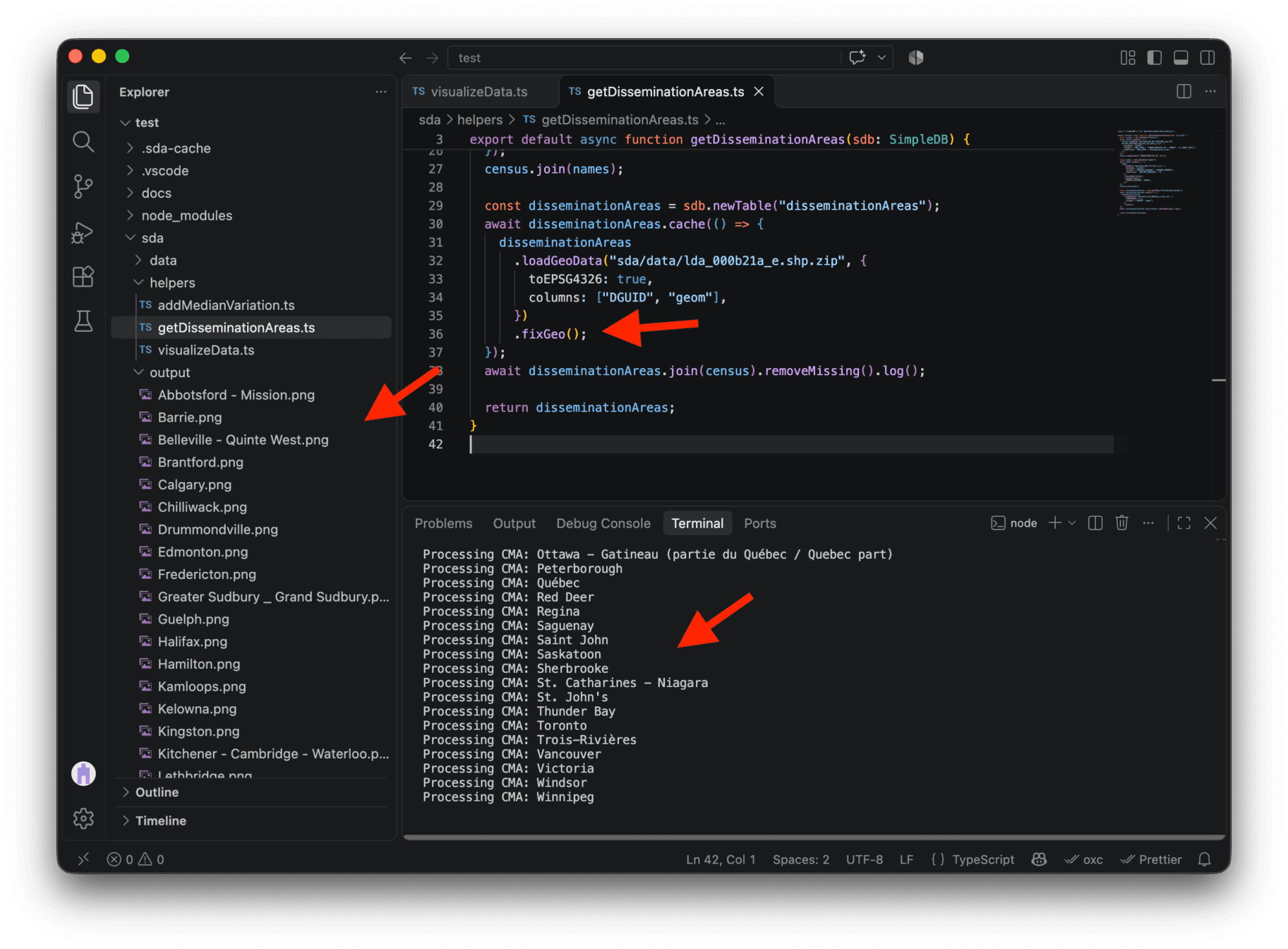
With the change saved, the script creates all 42 maps! 🥳 On my machine, this cached run took just seven seconds, which is impressive for creating so many maps.
These maps are PNG images. If you’d prefer editable vector files, change .png to .svg in the writeMap output path. You can then open the SVGs and tweak them in software like Illustrator.
Open a few images in sda/output to see the results. Montréal is my city, and I find the patterns of household income across it fascinating. Here’s its map at full resolution:
Conclusion
What a journey! Crunching big datasets with multiple tables storing tabular and geospatial data is not an easy task.
But I hope this real-life example showed you how you can cut through GB of data like it was butter with SDA. 🧈
To continue the course, head to Git & GitHub, where you’ll learn to track changes to your code and collaborate on projects.
Have fun with your next data project and feel free to reach out if you want to share what you are making with SDA or if you have any questions! 😊